9 Support Vector Machines

9.1 Conceptual

9.1.1 Question 1

This problem involves hyperplanes in two dimensions.

Sketch the hyperplane \(1 + 3X_1 − X_2 = 0\). Indicate the set of points for which \(1 + 3X_1 − X_2 > 0\), as well as the set of points for which \(1 + 3X_1 − X_2 < 0\).

library(ggplot2)
xlim <- c(-10, 10)
ylim <- c(-30, 30)
points <- expand.grid(
  X1 = seq(xlim[1], xlim[2], length.out = 50), 
  X2 = seq(ylim[1], ylim[2], length.out = 50)
)
p <- ggplot(points, aes(x = X1, y = X2)) + 
  geom_abline(intercept = 1, slope = 3) +  # X2 = 1 + 3X1 
  theme_bw()
p + geom_point(aes(color = 1 + 3*X1 - X2 > 0), size = 0.1) + 
  scale_color_discrete(name = "1 + 3X1 − X2 > 0")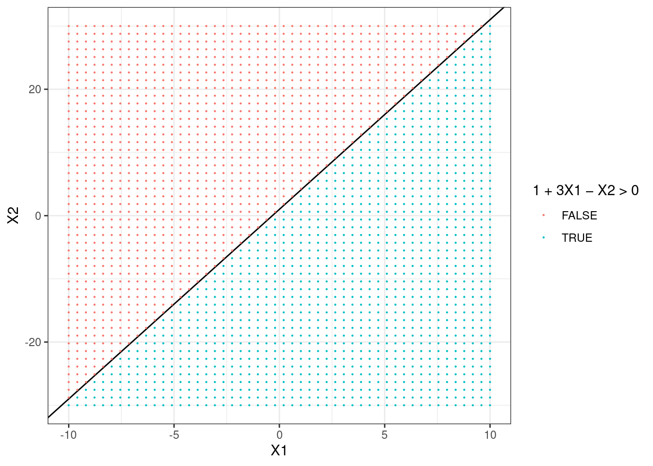

On the same plot, sketch the hyperplane \(−2 + X_1 + 2X_2 = 0\). Indicate the set of points for which \(−2 + X_1 + 2X_2 > 0\), as well as the set of points for which \(−2 + X_1 + 2X_2 < 0\).

p + geom_abline(intercept = 1, slope = -1/2) +  # X2 = 1 - X1/2
  geom_point(
    aes(color = interaction(1 + 3*X1 - X2 > 0, -2 + X1 + 2*X2 > 0)), 
    size = 0.5
  ) + 
  scale_color_discrete(name = "(1 + 3X1 − X2 > 0).(−2 + X1 + 2X2 > 0)")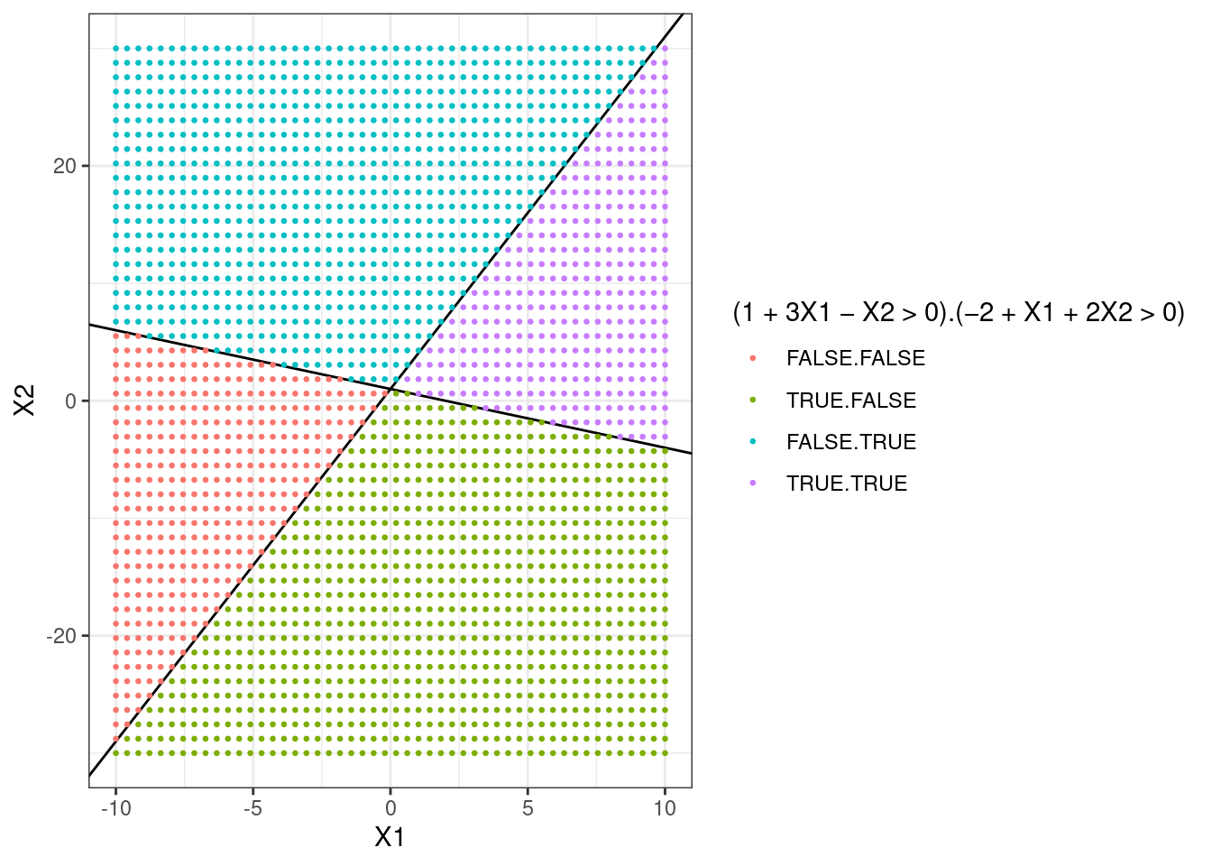

9.1.2 Question 2

We have seen that in \(p = 2\) dimensions, a linear decision boundary takes the form \(\beta_0 + \beta_1X_1 + \beta_2X_2 = 0\). We now investigate a non-linear decision boundary.

Sketch the curve \[(1+X_1)^2 +(2−X_2)^2 = 4\].

points <- expand.grid(
  X1 = seq(-4, 2, length.out = 100), 
  X2 = seq(-1, 5, length.out = 100)
)
p <- ggplot(points, aes(x = X1, y = X2, z = (1 + X1)^2 + (2 - X2)^2 - 4)) + 
  geom_contour(breaks = 0, colour = "black") + 
  theme_bw()
p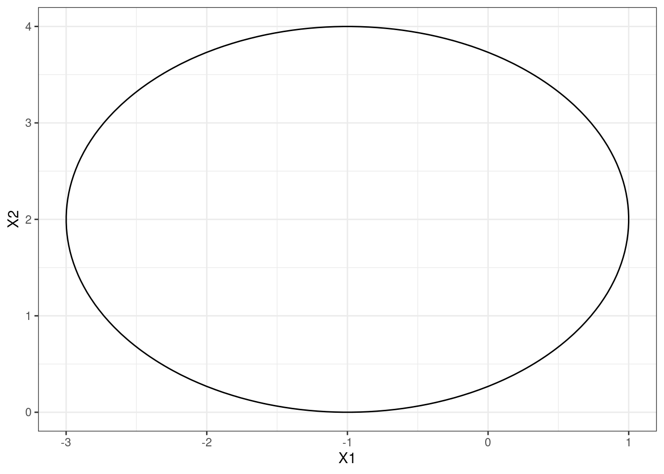

On your sketch, indicate the set of points for which \[(1 + X_1)^2 + (2 − X_2)^2 > 4,\] as well as the set of points for which \[(1 + X_1)^2 + (2 − X_2)^2 \leq 4.\]

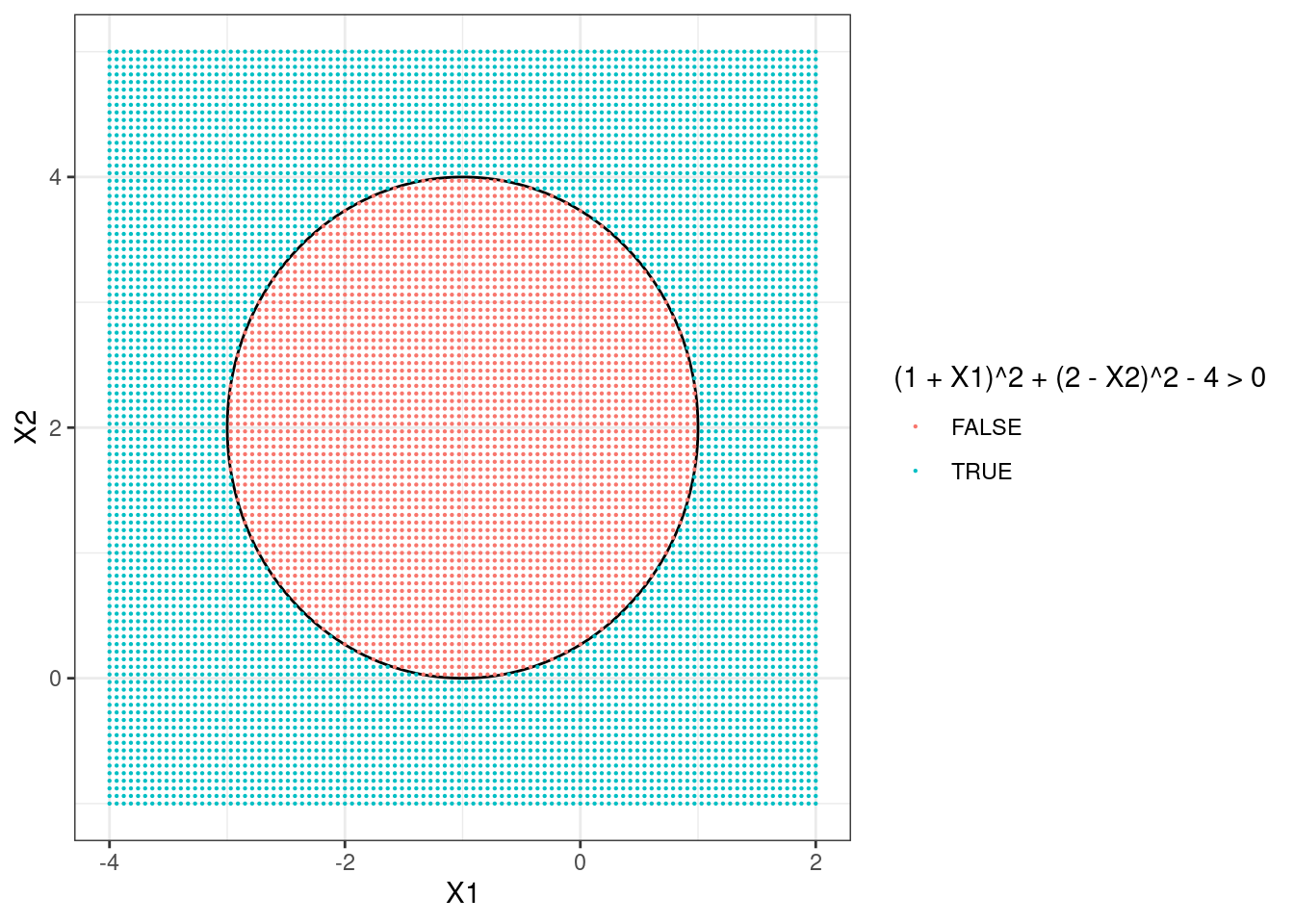
p + geom_point(aes(color = (1 + X1)^2 + (2 - X2)^2 - 4 > 0), size = 0.1)

Suppose that a classifier assigns an observation to the blue class if \[(1 + X_1)^2 + (2 − X_2)^2 > 4,\] and to the red class otherwise. To what class is the observation \((0, 0)\) classified? \((−1, 1)\)? \((2, 2)\)? \((3, 8)\)?

points <- data.frame(
  X1 = c(0, -1, 2, 3),
  X2 = c(0, 1, 2, 8)
)
ifelse((1 + points$X1)^2 + (2 - points$X2)^2 > 4, "blue", "red")

## [1] "blue" "red"  "blue" "blue"

Argue that while the decision boundary in (c) is not linear in terms of \(X_1\) and \(X_2\), it is linear in terms of \(X_1\), \(X_1^2\), \(X_2\), and \(X_2^2\).

The decision boundary is \[(1 + X_1)^2 + (2 − X_2)^2 -4 = 0\] which we can expand to: \[1 + 2X_1 + X_1^2 + 4 − 4X_2 + X_2^2 - 4 = 0\] which is linear in terms of \(X_1\), \(X_1^2\), \(X_2\), \(X_2^2\).

9.1.3 Question 3

Here we explore the maximal margin classifier on a toy data set.

We are given \(n = 7\) observations in \(p = 2\) dimensions. For each observation, there is an associated class label.

Obs. \(X_1\) \(X_2\) \(Y\)

1 3 4 Red

2 2 2 Red

3 4 4 Red

4 1 4 Red

5 2 1 Blue

6 4 3 Blue

7 4 1 Blue

Sketch the observations.

Obs.	\(X_1\)	\(X_2\)	\(Y\)
1	3	4	Red
2	2	2	Red
3	4	4	Red
4	1	4	Red
5	2	1	Blue
6	4	3	Blue
7	4	1	Blue

data <- data.frame(
  X1 = c(3, 2, 4, 1, 2, 4, 4),
  X2 = c(4, 2, 4, 4, 1, 3, 1),
  Y  = c(rep("Red", 4), rep("Blue", 3))
)
p <- ggplot(data, aes(x = X1, y = X2, color = Y)) + 
  geom_point(size = 2) + 
  scale_colour_identity() +
  coord_cartesian(xlim = c(0.5, 4.5), ylim = c(0.5, 4.5))
p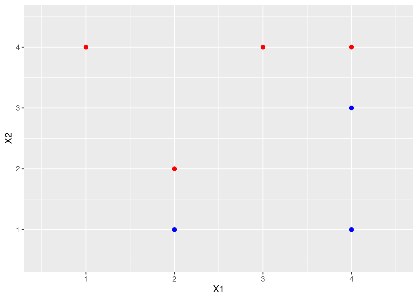

Sketch the optimal separating hyperplane, and provide the equation for this hyperplane (of the form (9.1)).

library(e1071)

fit <- svm(as.factor(Y) ~ ., data = data, kernel = "linear", cost = 10, scale = FALSE)

# Extract beta_0, beta_1, beta_2
beta <- c(
  -fit$rho,
  drop(t(fit$coefs) %*% as.matrix(data[fit$index, 1:2]))
)
names(beta) <- c("B0", "B1", "B2")
p <- p + geom_abline(intercept = -beta[1] / beta[3], slope = -beta[2] / beta[3], lty = 2)
p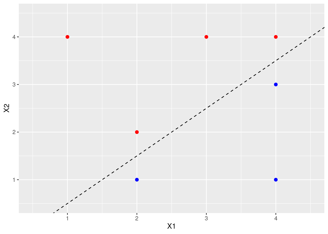

Describe the classification rule for the maximal margin classifier. It should be something along the lines of “Classify to Red if \(\beta_0 + \beta_1X_1 + \beta_2X_2 > 0\), and classify to Blue otherwise.” Provide the values for \(\beta_0, \beta_1,\) and \(\beta_2\).

Classify to red if \(\beta_0 + \beta_1X_1 + \beta_2X_2 > 0\) and blue otherwise where \(\beta_0 = 1\), \(\beta_1 = -2\), \(\beta_2 = 2\).

On your sketch, indicate the margin for the maximal margin hyperplane.

p <- p + geom_ribbon(
  aes(x = x, ymin = ymin, ymax = ymax),
  data = data.frame(x = c(0, 5), ymin = c(-1, 4), ymax = c(0, 5)),
  alpha = 0.1, fill = "blue",
  inherit.aes = FALSE
)
p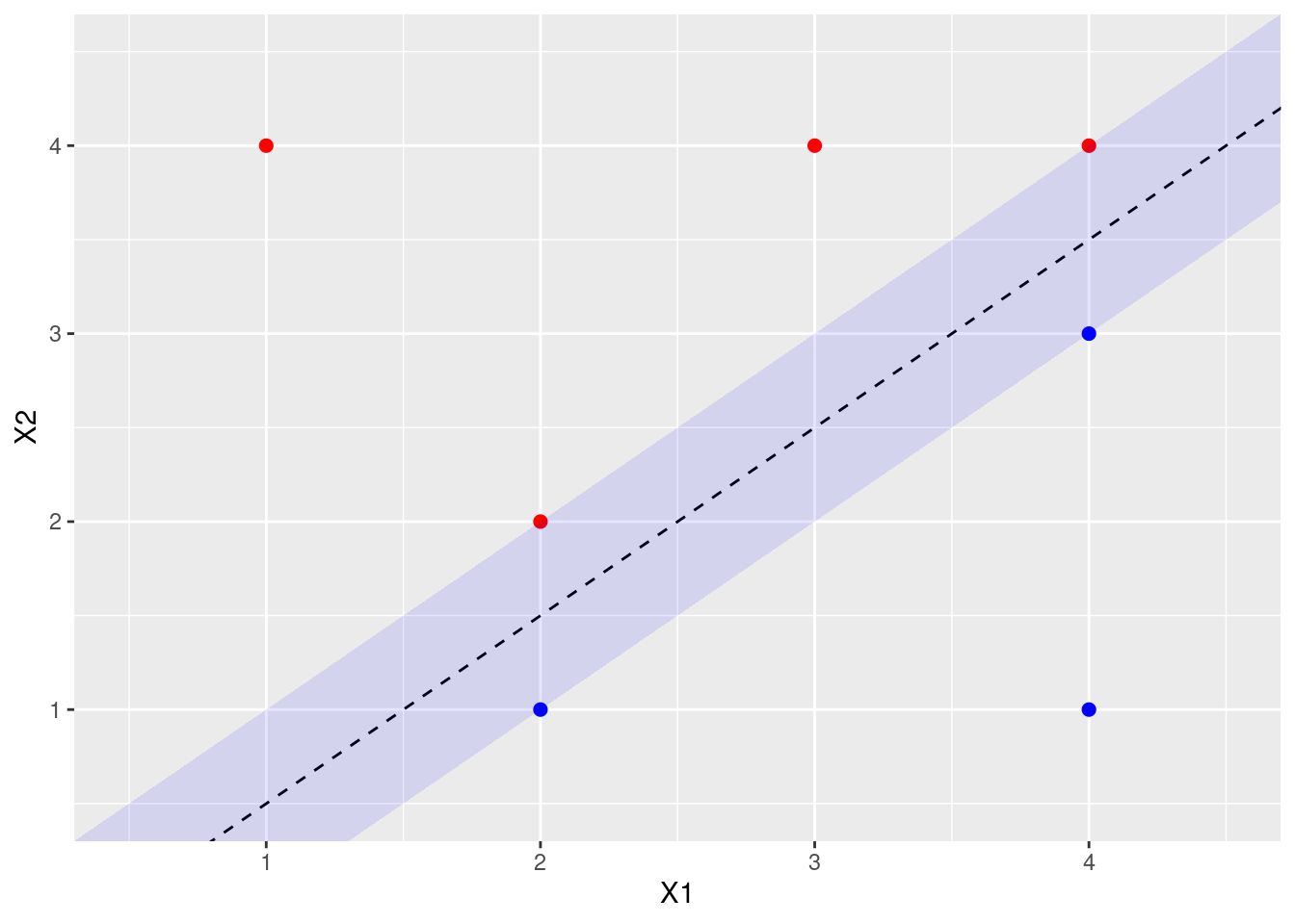

Indicate the support vectors for the maximal margin classifier.

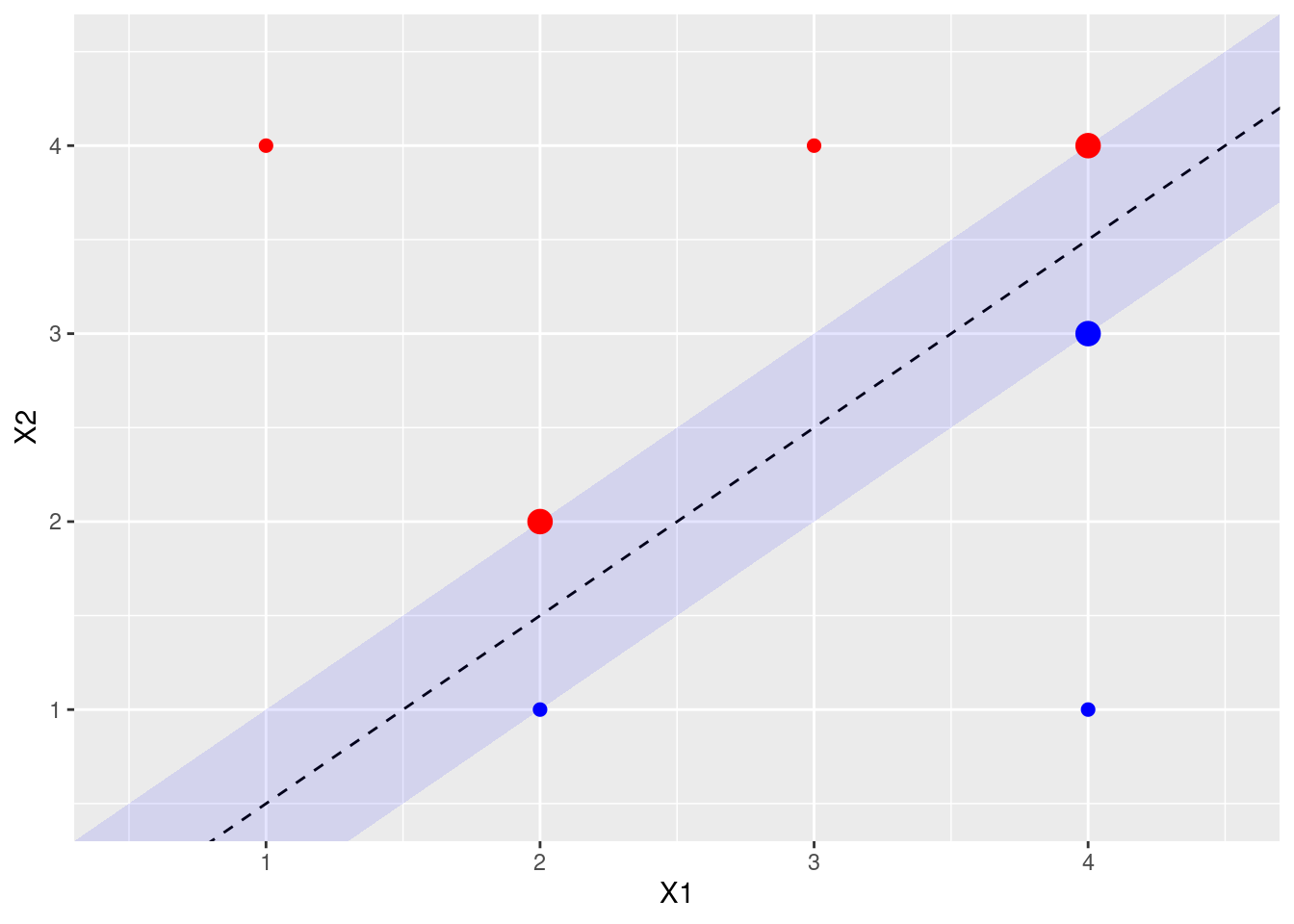
p <- p + geom_point(data = data[fit$index, ], size = 4)
p

The support vectors (from the svm fit object) are shown above. Arguably, there’s another support vector, since four points exactly touch the margin.

Argue that a slight movement of the seventh observation would not affect the maximal margin hyperplane.

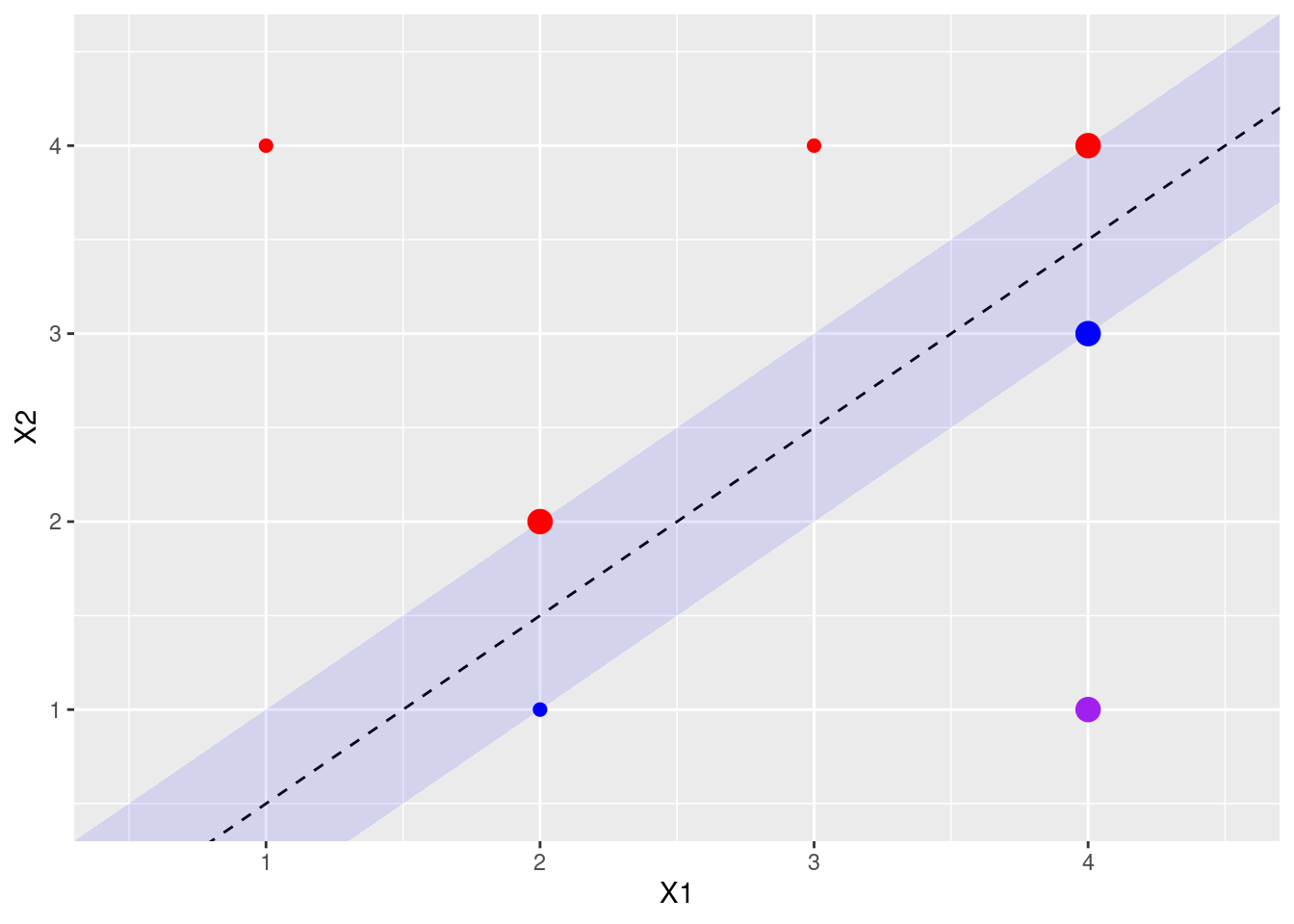
p + geom_point(data = data[7, , drop = FALSE], size = 4, color = "purple")

The 7th point is shown in purple above. It is not a support vector, and not close to the margin, so small changes in its X1, X2 values would not affect the current calculated margin.

Sketch a hyperplane that is not the optimal separating hyperplane, and provide the equation for this hyperplane.

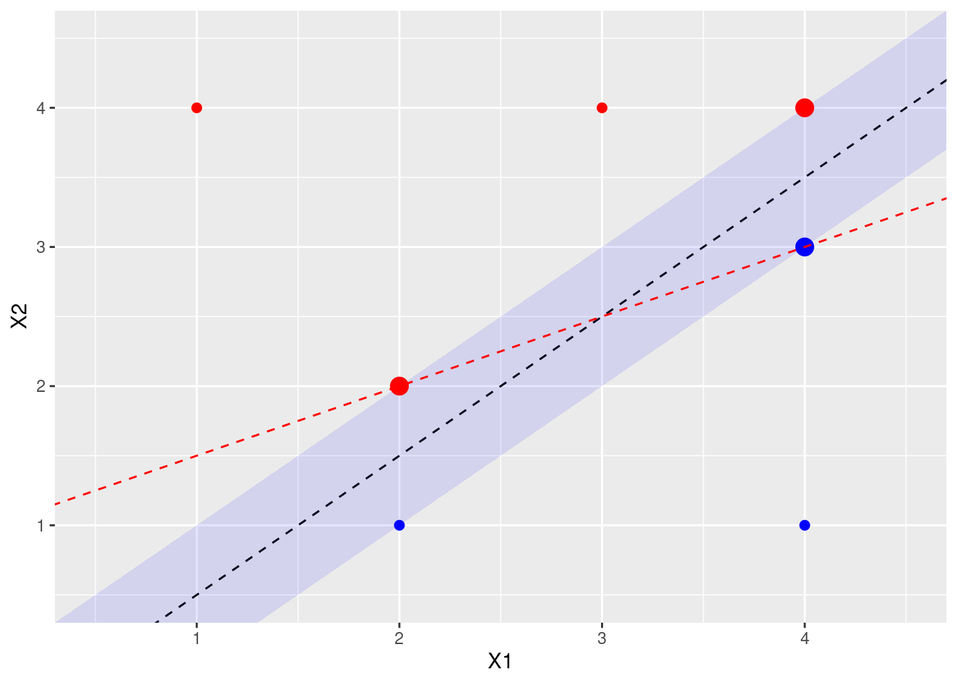
A non-optimal hyperline that still separates the blue and red points would be one that touches the (red) point at X1 = 2, X2 = 2 and the (blue) point at X1 = 4, X2 = 3. This gives line \(y = x/2 + 1\) or, when \(\beta_0 = -1\), \(\beta_1 = -1/2\), \(\beta_2 = 1\).

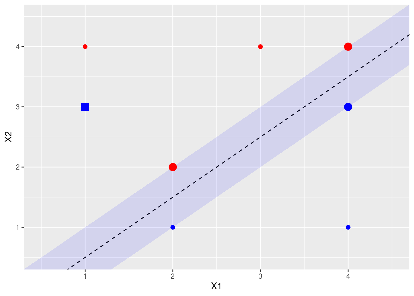
p + geom_abline(intercept = 1, slope = 0.5, lty = 2, col = "red")

Draw an additional observation on the plot so that the two classes are no longer separable by a hyperplane.

p + geom_point(data = data.frame(X1 = 1, X2 = 3, Y  = "Blue"), shape = 15, size = 4)

9.2 Applied

9.2.1 Question 4

Generate a simulated two-class data set with 100 observations and two features in which there is a visible but non-linear separation between the two classes. Show that in this setting, a support vector machine with a polynomial kernel (with degree greater than 1) or a radial kernel will outperform a support vector classifier on the training data. Which technique performs best on the test data? Make plots and report training and test error rates in order to back up your assertions.

set.seed(10)
data <- data.frame(
  x = runif(100),
  y = runif(100)
)
score <- (2*data$x-0.5)^2 + (data$y)^2 - 0.5
data$class <- factor(ifelse(score > 0, "red", "blue"))

p <- ggplot(data, aes(x = x, y = y, color = class)) + 
  geom_point(size = 2) + scale_colour_identity()
p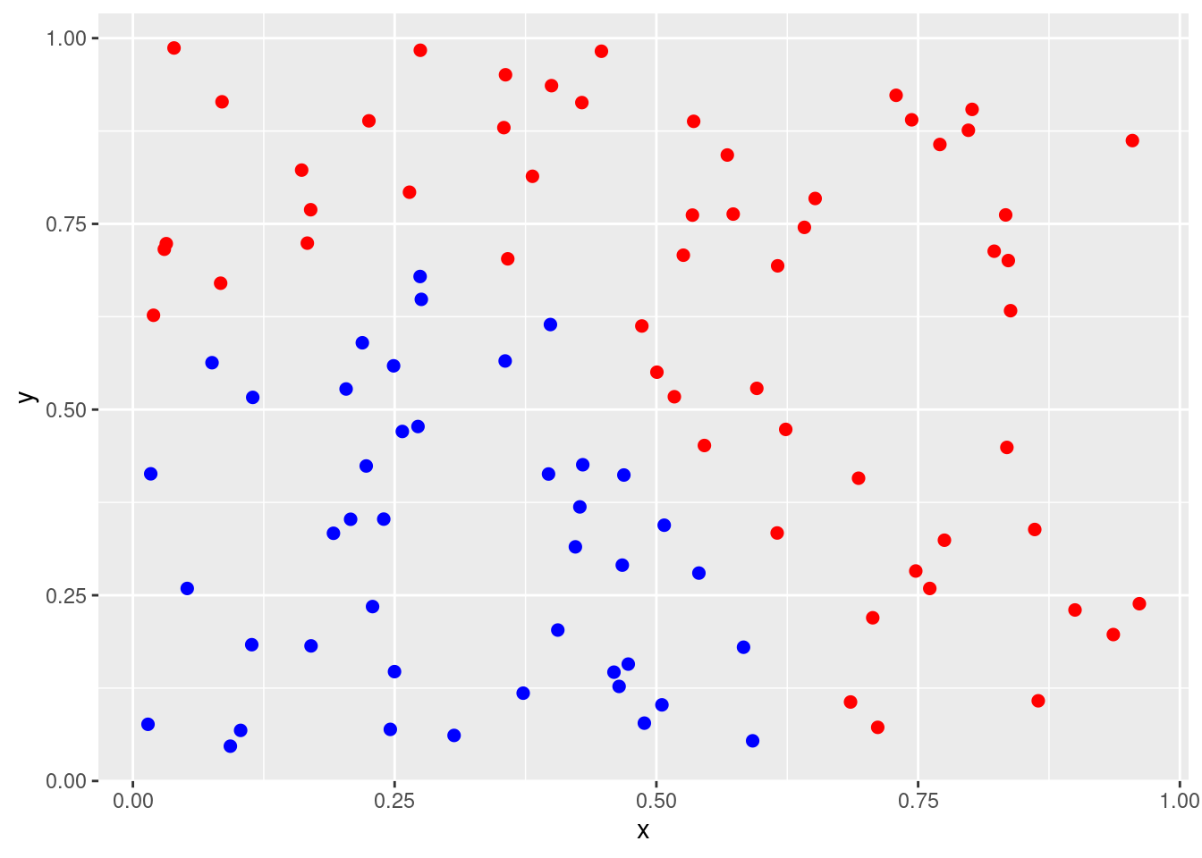

train <- 1:50
test <- 51:100

fits <- list(
  "Radial" = svm(class ~ ., data = data[train, ], kernel = "radial"),
  "Polynomial" = svm(class ~ ., data = data[train, ], kernel = "polynomial", degree = 2),
  "Linear" = svm(class ~ ., data = data[train, ], kernel = "linear")
)

err <- function(model, data) {
  out <- table(predict(model, data), data$class)
  (out[1, 2] + out[2, 1]) / sum(out)
}
plot(fits[[1]], data)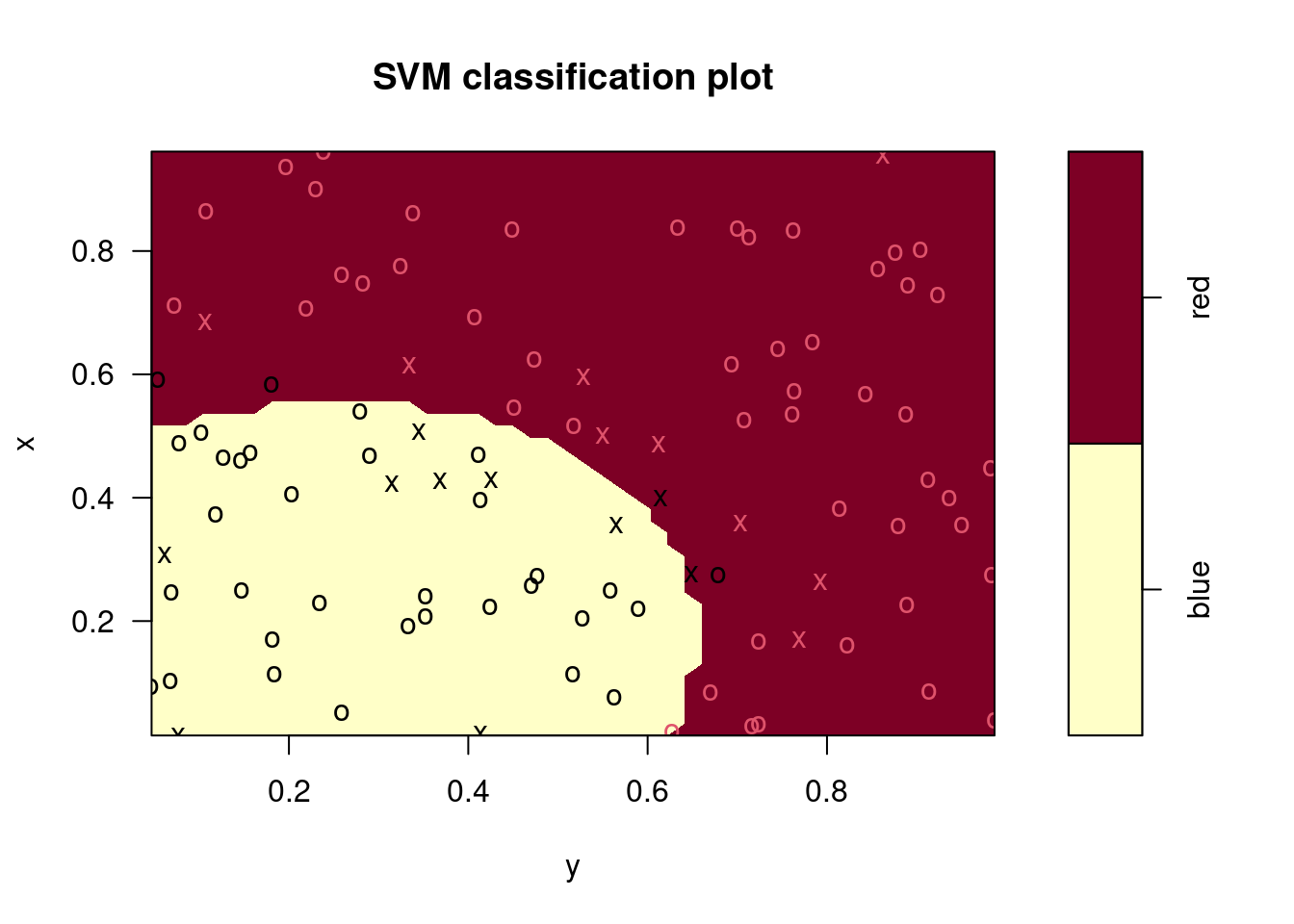

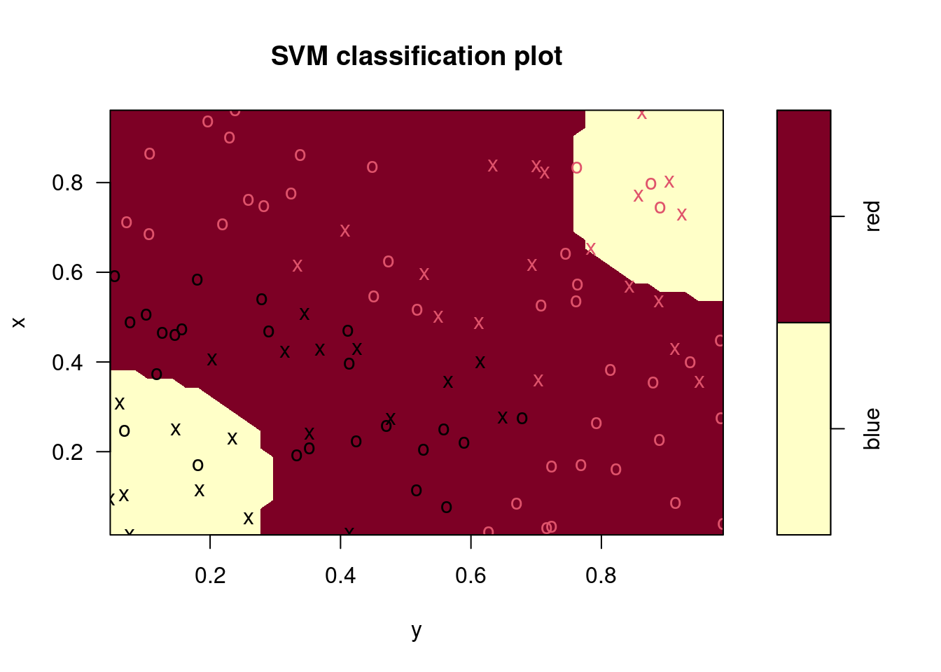
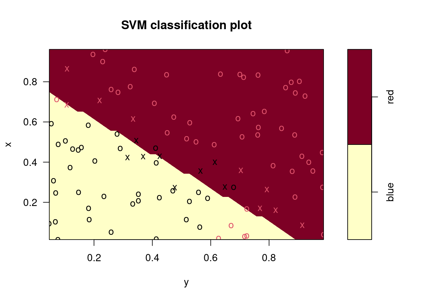
plot(fits[[2]], data)

plot(fits[[3]], data)

sapply(fits, err, data = data[train, ])

##     Radial Polynomial     Linear 
##       0.04       0.30       0.10

sapply(fits, err, data = data[test, ])

##     Radial Polynomial     Linear 
##       0.06       0.48       0.14

In this case, the radial kernel performs best, followed by a linear kernel with the 2nd degree polynomial performing worst. The ordering of these models is the same for the training and test data sets.

9.2.2 Question 5

We have seen that we can fit an SVM with a non-linear kernel in order to perform classification using a non-linear decision boundary. We will now see that we can also obtain a non-linear decision boundary by performing logistic regression using non-linear transformations of the features.
Generate a data set with \(n = 500\) and \(p = 2\), such that the observations belong to two classes with a quadratic decision boundary between them. For instance, you can do this as follows:
> x1 <- runif(500) - 0.5
> x2 <- runif(500) - 0.5
> y <- 1 * (x1^2 - x2^2 > 0)

set.seed(42)
train <- data.frame(
  x1 = runif(500) - 0.5,
  x2 = runif(500) - 0.5
)
train$y <- factor(as.numeric((train$x1^2 - train$x2^2 > 0)))

Plot the observations, colored according to their class labels. Your plot should display \(X_1\) on the \(x\)-axis, and \(X_2\) on the \(y\)-axis.

p <- ggplot(train, aes(x = x1, y = x2, color = y)) + 
  geom_point(size = 2)
p

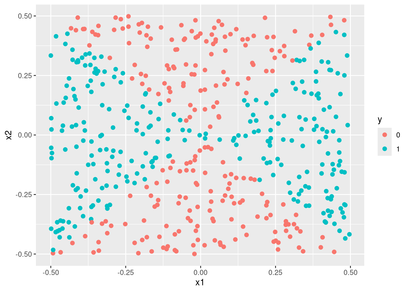
Fit a logistic regression model to the data, using \(X_1\) and \(X_2\) as predictors.

fit1 <- glm(y ~ ., data = train, family = "binomial")

Apply this model to the training data in order to obtain a predicted class label for each training observation. Plot the observations, colored according to the predicted class labels. The decision boundary should be linear.

plot_model <- function(fit) {
  if (inherits(fit, "svm")) {
    train$p <- predict(fit)
  } else {
    train$p <- factor(as.numeric(predict(fit) > 0))
  }
  ggplot(train, aes(x = x1, y = x2, color = p)) + 
    geom_point(size = 2)
}

plot_model(fit1)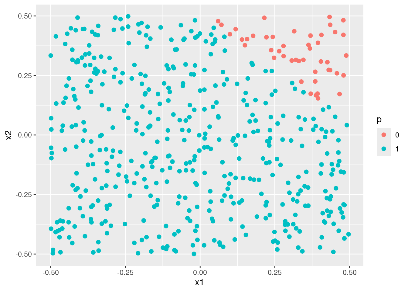

Now fit a logistic regression model to the data using non-linear functions of \(X_1\) and \(X_2\) as predictors (e.g. \(X_1^2, X_1 \times X_2, \log(X_2),\) and so forth).

fit2 <- glm(y ~ poly(x1, 2) + poly(x2, 2), data = train, family = "binomial")

## Warning: glm.fit: algorithm did not converge

## Warning: glm.fit: fitted probabilities numerically 0 or 1 occurred

Apply this model to the training data in order to obtain a predicted class label for each training observation. Plot the observations, colored according to the predicted class labels. The decision boundary should be obviously non-linear. If it is not, then repeat (a)-(e) until you come up with an example in which the predicted class labels are obviously non-linear.

plot_model(fit2)

Fit a support vector classifier to the data with \(X_1\) and \(X_2\) as predictors. Obtain a class prediction for each training observation. Plot the observations, colored according to the predicted class labels.

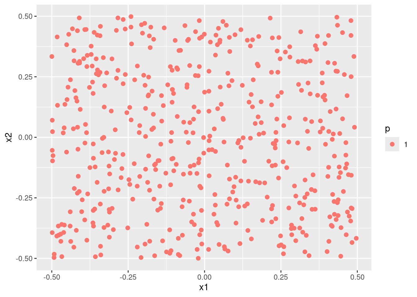
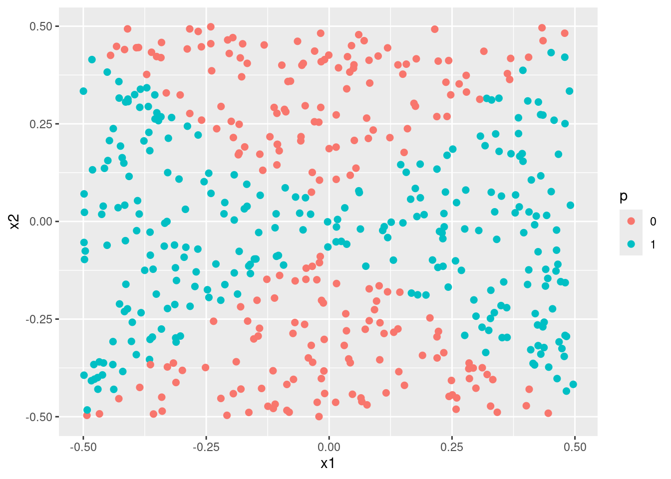
fit3 <- svm(y ~ x1 + x2, data = train, kernel = "linear")
plot_model(fit3)

Fit a SVM using a non-linear kernel to the data. Obtain a class prediction for each training observation. Plot the observations, colored according to the predicted class labels.

fit4 <- svm(y ~ x1 + x2, data = train, kernel = "polynomial", degree = 2)
plot_model(fit4)

Comment on your results.

When simulating data with a quadratic decision boundary, a logistic model with quadratic transformations of the variables and an svm model with a quadratic kernel both produce much better (and similar fits) than standard linear methods.

9.2.3 Question 6

At the end of Section 9.6.1, it is claimed that in the case of data that is just barely linearly separable, a support vector classifier with a small value of cost that misclassifies a couple of training observations may perform better on test data than one with a huge value of cost that does not misclassify any training observations. You will now investigate this claim.

Generate two-class data with \(p = 2\) in such a way that the classes are just barely linearly separable.

set.seed(2)

# Simulate data that is separable by a line at y = 2.5
data <- data.frame(
  x = rnorm(200),
  class = sample(c("red", "blue"), 200, replace = TRUE)
)
data$y <- (data$class == "red") * 5 + rnorm(200)

# Add barley separable points (these are simulated "noise" values)
newdata <- data.frame(x = rnorm(30))
newdata$y <- 1.5*newdata$x + 3 + rnorm(30, 0, 1)
newdata$class = ifelse((1.5*newdata$x + 3) - newdata$y > 0, "blue", "red")

data <- rbind(data, newdata)

# remove any that cause misclassification leaving data that is barley linearly
# separable, but along an axis that is not y = 2.5 (which would be correct
# for the "true" data.
data <- data[!(data$class == "red") == ((1.5*data$x + 3 - data$y) > 0), ]
data <- data[sample(seq_len(nrow(data)), 200), ]

p <- ggplot(data, aes(x = x, y = y, color = class)) + 
  geom_point(size = 2) + scale_colour_identity() + 
  geom_abline(intercept = 3, slope = 1.5, lty = 2)
p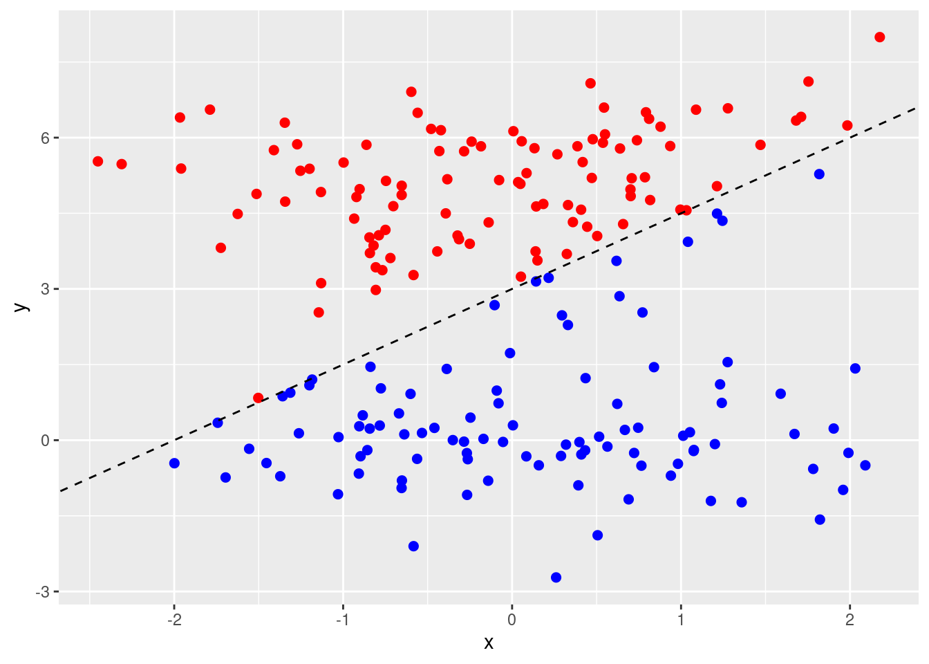

Compute the cross-validation error rates for support vector classifiers with a range of cost values. How many training errors are misclassified for each value of cost considered, and how does this relate to the cross-validation errors obtained?

How many training errors are misclassified for each value of cost?

costs <- 10^seq(-3, 5)

sapply(costs, function(cost) {
    fit <- svm(as.factor(class) ~ ., data = data, kernel = "linear", cost = cost)
    pred <- predict(fit, data)
    sum(pred != data$class)
})

## [1] 98  8  9  4  1  1  0  0  0

Cross-validation errors

out <- tune(svm, as.factor(class) ~ ., data = data, kernel = "linear", ranges = list(cost = costs))
summary(out)

## 
## Parameter tuning of 'svm':
## 
## - sampling method: 10-fold cross validation 
## 
## - best parameters:
##  cost
##    10
## 
## - best performance: 0.005 
## 
## - Detailed performance results:
##    cost error dispersion
## 1 1e-03 0.540 0.09067647
## 2 1e-02 0.045 0.02838231
## 3 1e-01 0.045 0.03689324
## 4 1e+00 0.020 0.02581989
## 5 1e+01 0.005 0.01581139
## 6 1e+02 0.005 0.01581139
## 7 1e+03 0.005 0.01581139
## 8 1e+04 0.010 0.02108185
## 9 1e+05 0.010 0.02108185

data.frame(
  cost = out$performances$cost, 
  misclass = out$performances$error * nrow(data)
)

##    cost misclass
## 1 1e-03      108
## 2 1e-02        9
## 3 1e-01        9
## 4 1e+00        4
## 5 1e+01        1
## 6 1e+02        1
## 7 1e+03        1
## 8 1e+04        2
## 9 1e+05        2

Generate an appropriate test data set, and compute the test errors corresponding to each of the values of cost considered. Which value of cost leads to the fewest test errors, and how does this compare to the values of cost that yield the fewest training errors and the fewest cross-validation errors?

set.seed(2)
test <- data.frame(
  x = rnorm(200),
  class = sample(c("red", "blue"), 200, replace = TRUE)
)
test$y <- (test$class == "red") * 5 + rnorm(200)
p + geom_point(data = test, pch = 21)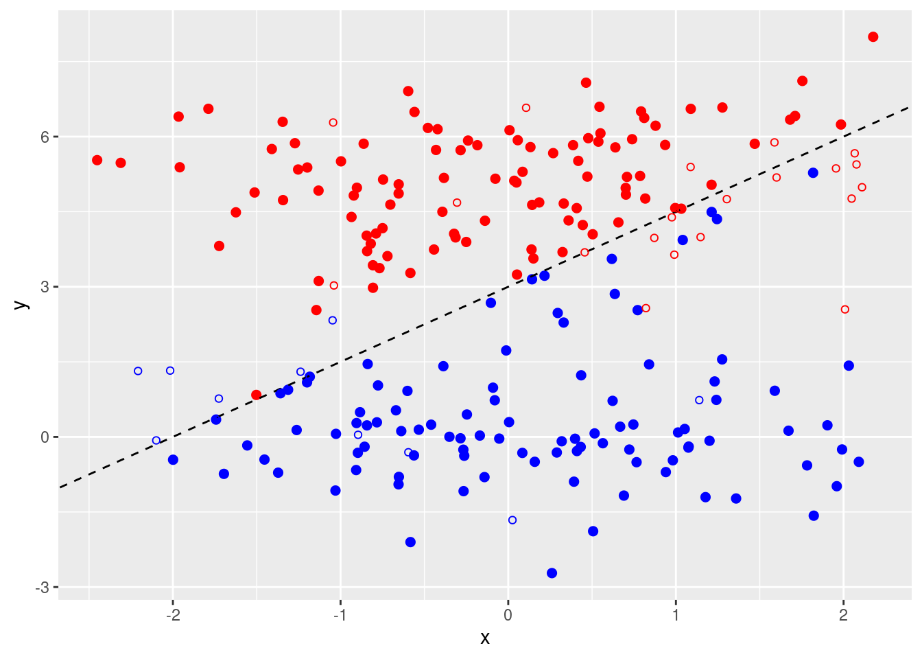

(errs <- sapply(costs, function(cost) {
    fit <- svm(as.factor(class) ~ ., data = data, kernel = "linear", cost = cost)
    pred <- predict(fit, test)
    sum(pred != test$class)
}))

## [1] 95  2  3  9 16 16 19 19 19

(cost <- costs[which.min(errs)])

## [1] 0.01

(fit <- svm(as.factor(class) ~ ., data = data, kernel = "linear", cost = cost))

## 
## Call:
## svm(formula = as.factor(class) ~ ., data = data, kernel = "linear", 
##     cost = cost)
## 
## 
## Parameters:
##    SVM-Type:  C-classification 
##  SVM-Kernel:  linear 
##        cost:  0.01 
## 
## Number of Support Vectors:  135

test$prediction <- predict(fit, test)
p <- ggplot(test, aes(x = x, y = y, color = class, shape = prediction == class)) + 
  geom_point(size = 2) + 
  scale_colour_identity() 
p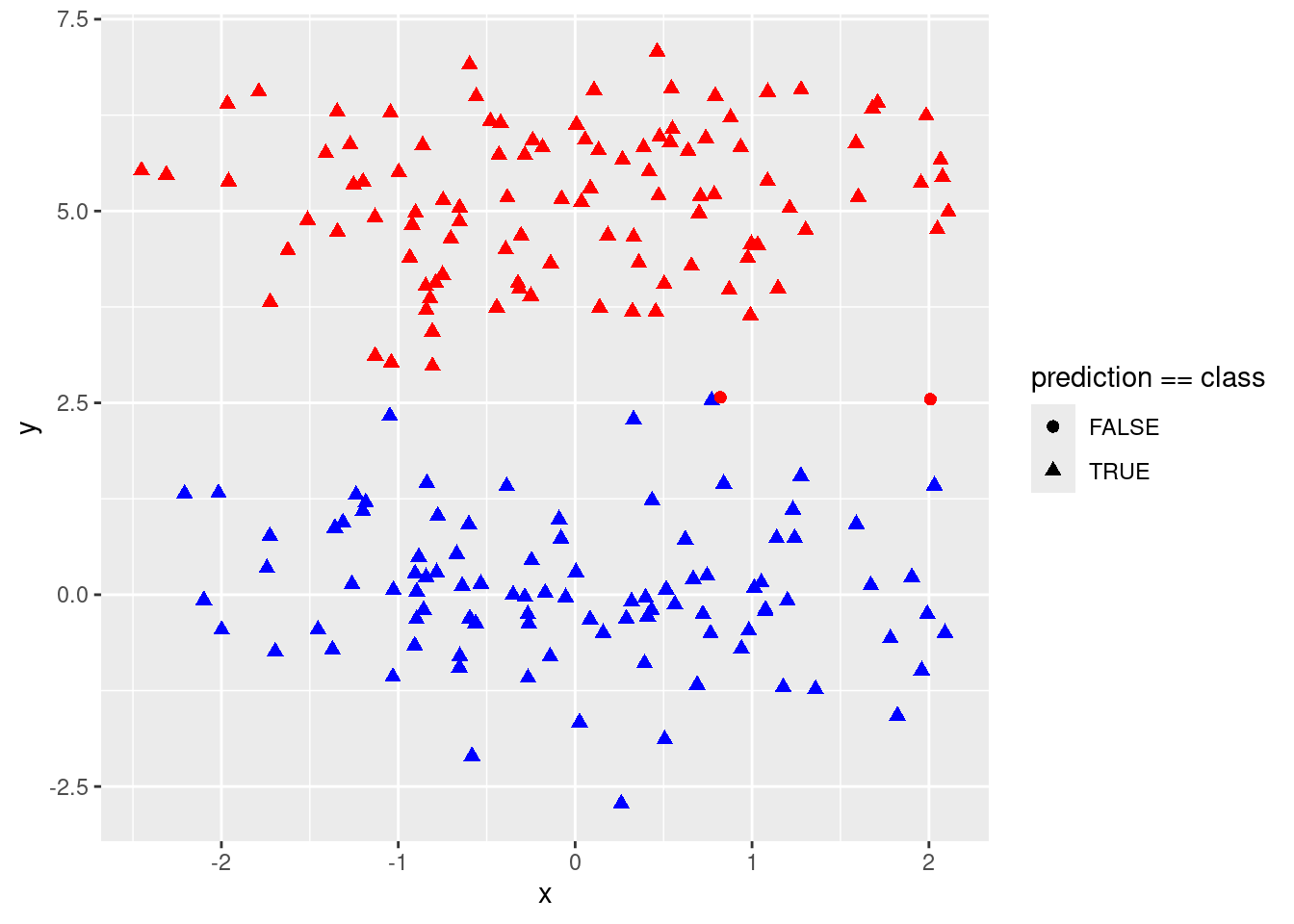

Discuss your results.

A large cost leads to overfitting as the model finds the perfect linear separation between red and blue in the training data. A lower cost then leads to improved prediction in the test data.

9.2.4 Question 7

In this problem, you will use support vector approaches in order to predict whether a given car gets high or low gas mileage based on the Auto data set.

Create a binary variable that takes on a 1 for cars with gas mileage above the median, and a 0 for cars with gas mileage below the median.

library(ISLR2)
data <- Auto
data$high_mpg <- as.factor(as.numeric(data$mpg > median(data$mpg)))

Fit a support vector classifier to the data with various values of cost, in order to predict whether a car gets high or low gas mileage. Report the cross-validation errors associated with different values of this parameter. Comment on your results. Note you will need to fit the classifier without the gas mileage variable to produce sensible results.

set.seed(42)
costs <- 10^seq(-4, 3, by = 0.5)
results <- list()
f <- high_mpg ~ displacement + horsepower + weight
results$linear <- tune(svm, f, data = data, kernel = "linear", 
  ranges = list(cost = costs))
summary(results$linear)

## 
## Parameter tuning of 'svm':
## 
## - sampling method: 10-fold cross validation 
## 
## - best parameters:
##        cost
##  0.03162278
## 
## - best performance: 0.1019231 
## 
## - Detailed performance results:
##            cost     error dispersion
## 1  1.000000e-04 0.5967949 0.05312225
## 2  3.162278e-04 0.5967949 0.05312225
## 3  1.000000e-03 0.2199359 0.08718077
## 4  3.162278e-03 0.1353846 0.06058195
## 5  1.000000e-02 0.1121795 0.04011293
## 6  3.162278e-02 0.1019231 0.05087176
## 7  1.000000e-01 0.1096154 0.05246238
## 8  3.162278e-01 0.1044872 0.05154934
## 9  1.000000e+00 0.1044872 0.05154934
## 10 3.162278e+00 0.1044872 0.05154934
## 11 1.000000e+01 0.1019231 0.05501131
## 12 3.162278e+01 0.1019231 0.05501131
## 13 1.000000e+02 0.1019231 0.05501131
## 14 3.162278e+02 0.1019231 0.05501131
## 15 1.000000e+03 0.1019231 0.05501131

Now repeat (b), this time using SVMs with radial and polynomial basis kernels, with different values of gamma and degree and cost. Comment on your results.

results$polynomial <- tune(svm, f, data = data, kernel = "polynomial", 
  ranges = list(cost = costs, degree = 1:3))
summary(results$polynomial)

## 
## Parameter tuning of 'svm':
## 
## - sampling method: 10-fold cross validation 
## 
## - best parameters:
##  cost degree
##   0.1      1
## 
## - best performance: 0.101859 
## 
## - Detailed performance results:
##            cost degree     error dispersion
## 1  1.000000e-04      1 0.5842949 0.04703306
## 2  3.162278e-04      1 0.5842949 0.04703306
## 3  1.000000e-03      1 0.5842949 0.04703306
## 4  3.162278e-03      1 0.2167949 0.07891173
## 5  1.000000e-02      1 0.1275641 0.04806885
## 6  3.162278e-02      1 0.1147436 0.05661708
## 7  1.000000e-01      1 0.1018590 0.05732429
## 8  3.162278e-01      1 0.1069231 0.05949679
## 9  1.000000e+00      1 0.1069231 0.06307278
## 10 3.162278e+00      1 0.1069231 0.06307278
## 11 1.000000e+01      1 0.1043590 0.06603760
## 12 3.162278e+01      1 0.1043590 0.06603760
## 13 1.000000e+02      1 0.1043590 0.06603760
## 14 3.162278e+02      1 0.1043590 0.06603760
## 15 1.000000e+03      1 0.1043590 0.06603760
## 16 1.000000e-04      2 0.5842949 0.04703306
## 17 3.162278e-04      2 0.5842949 0.04703306
## 18 1.000000e-03      2 0.5842949 0.04703306
## 19 3.162278e-03      2 0.5255128 0.08090636
## 20 1.000000e-02      2 0.3980769 0.08172400
## 21 3.162278e-02      2 0.3674359 0.07974741
## 22 1.000000e-01      2 0.3597436 0.08336609
## 23 3.162278e-01      2 0.3597436 0.09010398
## 24 1.000000e+00      2 0.3444872 0.08767258
## 25 3.162278e+00      2 0.3545513 0.10865903
## 26 1.000000e+01      2 0.3239103 0.09593710
## 27 3.162278e+01      2 0.3035256 0.08184137
## 28 1.000000e+02      2 0.3061538 0.08953945
## 29 3.162278e+02      2 0.3060897 0.08919821
## 30 1.000000e+03      2 0.3035897 0.09305216
## 31 1.000000e-04      3 0.5842949 0.04703306
## 32 3.162278e-04      3 0.4955128 0.10081350
## 33 1.000000e-03      3 0.3750641 0.08043982
## 34 3.162278e-03      3 0.3036538 0.09096445
## 35 1.000000e-02      3 0.2601282 0.07774595
## 36 3.162278e-02      3 0.2499359 0.08407106
## 37 1.000000e-01      3 0.2017949 0.07547413
## 38 3.162278e-01      3 0.1937179 0.08427411
## 39 1.000000e+00      3 0.1478205 0.04579654
## 40 3.162278e+00      3 0.1451923 0.05169638
## 41 1.000000e+01      3 0.1451282 0.04698931
## 42 3.162278e+01      3 0.1500000 0.07549058
## 43 1.000000e+02      3 0.1373718 0.05772558
## 44 3.162278e+02      3 0.1271795 0.06484766
## 45 1.000000e+03      3 0.1322436 0.06764841

results$radial <- tune(svm, f, data = data, kernel = "radial", 
  ranges = list(cost = costs, gamma = 10^(-2:1)))
summary(results$radial)

## 
## Parameter tuning of 'svm':
## 
## - sampling method: 10-fold cross validation 
## 
## - best parameters:
##  cost gamma
##  1000   0.1
## 
## - best performance: 0.08179487 
## 
## - Detailed performance results:
##            cost gamma      error dispersion
## 1  1.000000e-04  0.01 0.58410256 0.05435320
## 2  3.162278e-04  0.01 0.58410256 0.05435320
## 3  1.000000e-03  0.01 0.58410256 0.05435320
## 4  3.162278e-03  0.01 0.58410256 0.05435320
## 5  1.000000e-02  0.01 0.58410256 0.05435320
## 6  3.162278e-02  0.01 0.26557692 0.10963269
## 7  1.000000e-01  0.01 0.15038462 0.05783237
## 8  3.162278e-01  0.01 0.11224359 0.04337812
## 9  1.000000e+00  0.01 0.10730769 0.04512161
## 10 3.162278e+00  0.01 0.10730769 0.04512161
## 11 1.000000e+01  0.01 0.10737179 0.05526490
## 12 3.162278e+01  0.01 0.10480769 0.05610124
## 13 1.000000e+02  0.01 0.10480769 0.05610124
## 14 3.162278e+02  0.01 0.10737179 0.05526490
## 15 1.000000e+03  0.01 0.10993590 0.05690926
## 16 1.000000e-04  0.10 0.58410256 0.05435320
## 17 3.162278e-04  0.10 0.58410256 0.05435320
## 18 1.000000e-03  0.10 0.58410256 0.05435320
## 19 3.162278e-03  0.10 0.58410256 0.05435320
## 20 1.000000e-02  0.10 0.15301282 0.06026554
## 21 3.162278e-02  0.10 0.11480769 0.04514816
## 22 1.000000e-01  0.10 0.10730769 0.04512161
## 23 3.162278e-01  0.10 0.10730769 0.04512161
## 24 1.000000e+00  0.10 0.10737179 0.05526490
## 25 3.162278e+00  0.10 0.10737179 0.05526490
## 26 1.000000e+01  0.10 0.10737179 0.05526490
## 27 3.162278e+01  0.10 0.10737179 0.05526490
## 28 1.000000e+02  0.10 0.09967949 0.04761387
## 29 3.162278e+02  0.10 0.08429487 0.03207585
## 30 1.000000e+03  0.10 0.08179487 0.03600437
## 31 1.000000e-04  1.00 0.58410256 0.05435320
## 32 3.162278e-04  1.00 0.58410256 0.05435320
## 33 1.000000e-03  1.00 0.58410256 0.05435320
## 34 3.162278e-03  1.00 0.58410256 0.05435320
## 35 1.000000e-02  1.00 0.12506410 0.05342773
## 36 3.162278e-02  1.00 0.10730769 0.06255920
## 37 1.000000e-01  1.00 0.10993590 0.05561080
## 38 3.162278e-01  1.00 0.10737179 0.05526490
## 39 1.000000e+00  1.00 0.09711538 0.05107441
## 40 3.162278e+00  1.00 0.08429487 0.03634646
## 41 1.000000e+01  1.00 0.08692308 0.03877861
## 42 3.162278e+01  1.00 0.08948718 0.03503648
## 43 1.000000e+02  1.00 0.09198718 0.03272127
## 44 3.162278e+02  1.00 0.10217949 0.04214031
## 45 1.000000e+03  1.00 0.09692308 0.04645046
## 46 1.000000e-04 10.00 0.58410256 0.05435320
## 47 3.162278e-04 10.00 0.58410256 0.05435320
## 48 1.000000e-03 10.00 0.58410256 0.05435320
## 49 3.162278e-03 10.00 0.58410256 0.05435320
## 50 1.000000e-02 10.00 0.58410256 0.05435320
## 51 3.162278e-02 10.00 0.22205128 0.12710181
## 52 1.000000e-01 10.00 0.11237179 0.03888895
## 53 3.162278e-01 10.00 0.10217949 0.04375722
## 54 1.000000e+00 10.00 0.09717949 0.03809440
## 55 3.162278e+00 10.00 0.09717949 0.03809440
## 56 1.000000e+01 10.00 0.09711538 0.04161705
## 57 3.162278e+01 10.00 0.11487179 0.04240664
## 58 1.000000e+02 10.00 0.13019231 0.03541140
## 59 3.162278e+02 10.00 0.13532051 0.03865626
## 60 1.000000e+03 10.00 0.14044872 0.04251917

sapply(results, function(x) x$best.performance)

##     linear polynomial     radial 
## 0.10192308 0.10185897 0.08179487

sapply(results, function(x) x$best.parameters)

## $linear
##         cost
## 6 0.03162278
## 
## $polynomial
##   cost degree
## 7  0.1      1
## 
## $radial
##    cost gamma
## 30 1000   0.1

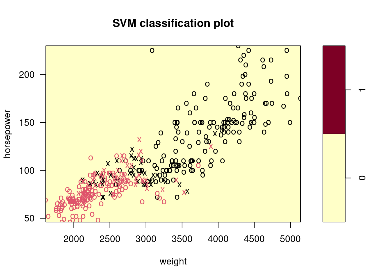
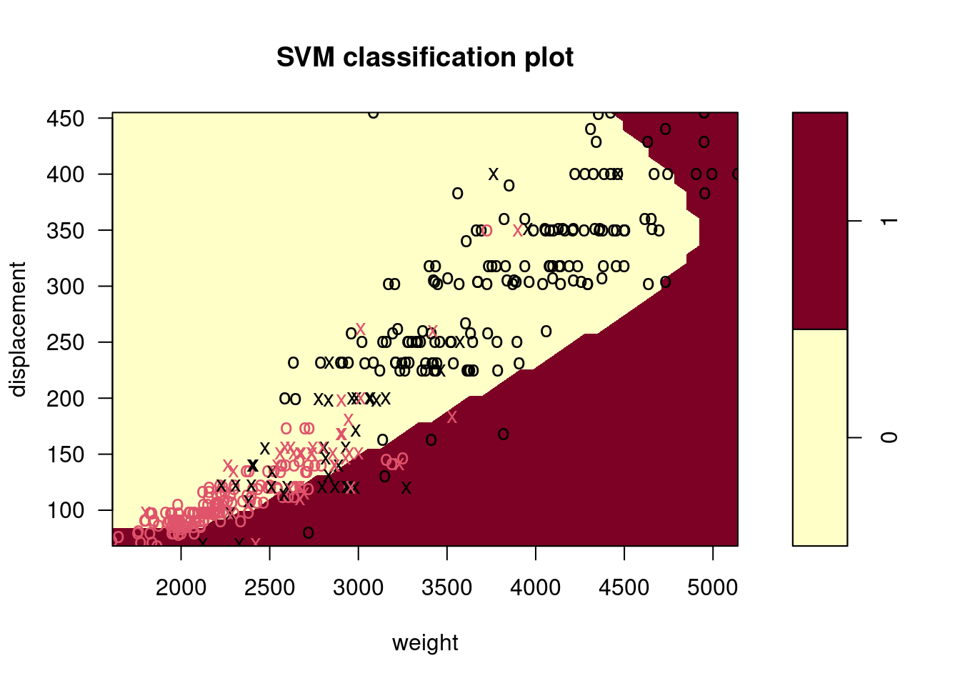
Make some plots to back up your assertions in (b) and (c).

Hint: In the lab, we used the plot() function for svm objects only in cases with \(p = 2\). When \(p > 2\), you can use the plot() function to create plots displaying pairs of variables at a time. Essentially, instead of typing
> plot(svmfit, dat)
where svmfit contains your fitted model and dat is a data frame containing your data, you can type
> plot(svmfit, dat, x1 ∼ x4)
in order to plot just the first and fourth variables. However, you must replace x1 and x4 with the correct variable names. To find out more, type ?plot.svm.

table(predict(results$radial$best.model, data), data$high_mpg)

##    
##       0   1
##   0 176   5
##   1  20 191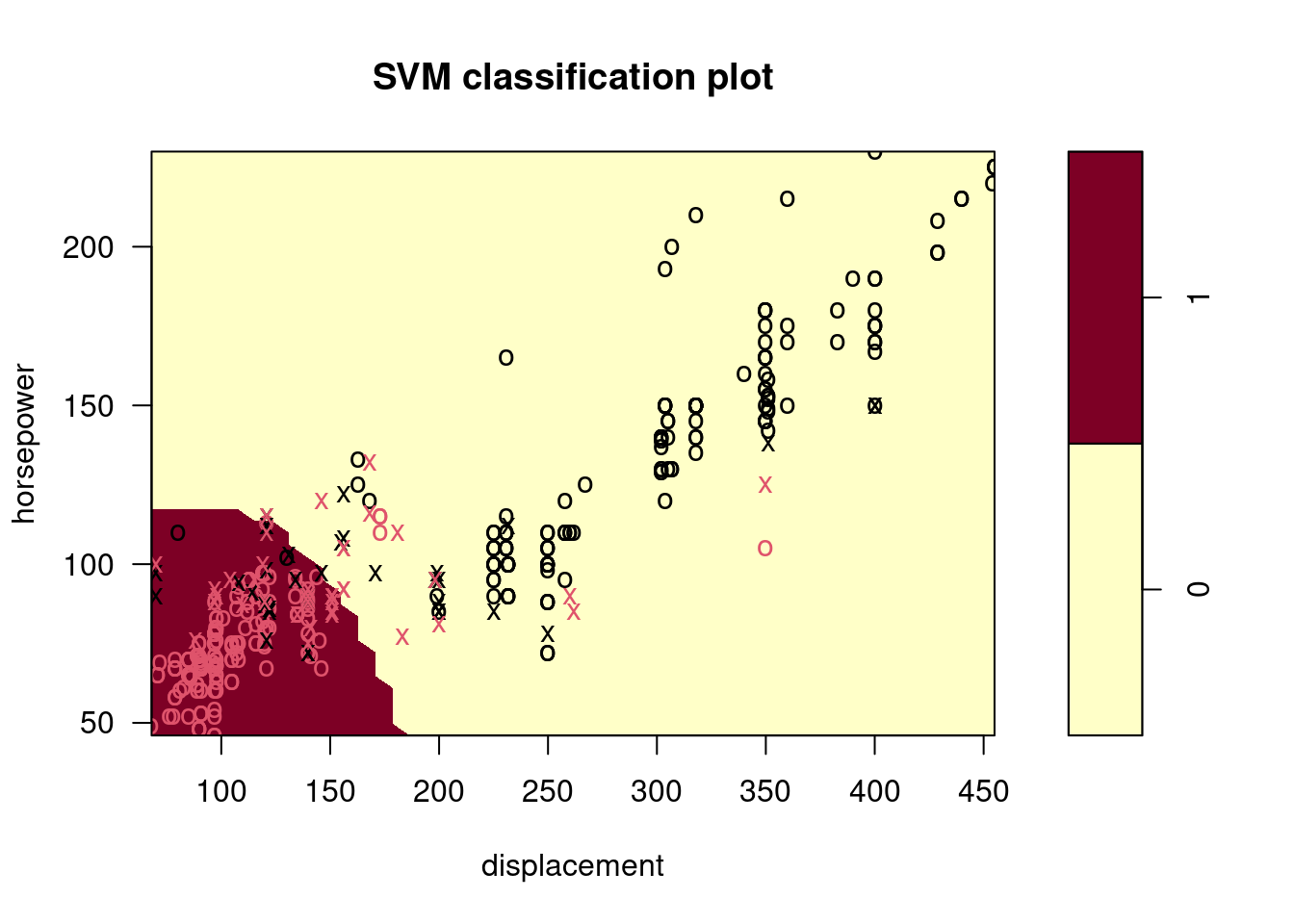

plot(results$radial$best.model, data, horsepower~displacement)

plot(results$radial$best.model, data, horsepower~weight)

plot(results$radial$best.model, data, displacement~weight)

9.2.5 Question 8

This problem involves the OJ data set which is part of the ISLR2 package.

Create a training set containing a random sample of 800 observations, and a test set containing the remaining observations.

set.seed(42)
train <- sample(seq_len(nrow(OJ)), 800)
test <- setdiff(seq_len(nrow(OJ)), train)

Fit a support vector classifier to the training data using cost = 0.01, with Purchase as the response and the other variables as predictors. Use the summary() function to produce summary statistics, and describe the results obtained.

fit <- svm(Purchase ~ ., data = OJ[train, ], kernel = "linear", cost = 0.01)
summary(fit)

## 
## Call:
## svm(formula = Purchase ~ ., data = OJ[train, ], kernel = "linear", 
##     cost = 0.01)
## 
## 
## Parameters:
##    SVM-Type:  C-classification 
##  SVM-Kernel:  linear 
##        cost:  0.01 
## 
## Number of Support Vectors:  432
## 
##  ( 215 217 )
## 
## 
## Number of Classes:  2 
## 
## Levels: 
##  CH MM

What are the training and test error rates?

err <- function(model, data) {
  t <- table(predict(model, data), data[["Purchase"]])
  1 - sum(diag(t)) / sum(t)
}
errs <- function(model) {
  c(train = err(model, OJ[train, ]), test = err(model, OJ[test, ]))
}
errs(fit)

##    train     test 
## 0.171250 0.162963

Use the tune() function to select an optimal cost. Consider values in the range 0.01 to 10.

tuned <- tune(svm, Purchase ~ ., data = OJ[train, ], kernel = "linear", 
  ranges = list(cost = 10^seq(-2, 1, length.out = 10)))
tuned$best.parameters

##   cost
## 7    1

summary(tuned)

## 
## Parameter tuning of 'svm':
## 
## - sampling method: 10-fold cross validation 
## 
## - best parameters:
##  cost
##     1
## 
## - best performance: 0.1775 
## 
## - Detailed performance results:
##           cost   error dispersion
## 1   0.01000000 0.18250 0.04133199
## 2   0.02154435 0.18000 0.04005205
## 3   0.04641589 0.18000 0.05041494
## 4   0.10000000 0.18000 0.04901814
## 5   0.21544347 0.18250 0.04377975
## 6   0.46415888 0.18250 0.04090979
## 7   1.00000000 0.17750 0.04031129
## 8   2.15443469 0.18000 0.03961621
## 9   4.64158883 0.17875 0.03821086
## 10 10.00000000 0.18375 0.03438447

Compute the training and test error rates using this new value for cost.

errs(tuned$best.model)

##    train     test 
## 0.167500 0.162963

Repeat parts (b) through (e) using a support vector machine with a radial kernel. Use the default value for gamma.

tuned2 <- tune(svm, Purchase ~ ., data = OJ[train, ], kernel = "radial", 
  ranges = list(cost = 10^seq(-2, 1, length.out = 10)))
tuned2$best.parameters

##        cost
## 6 0.4641589

errs(tuned2$best.model)

##     train      test 
## 0.1525000 0.1666667

Repeat parts (b) through (e) using a support vector machine with a polynomial kernel. Set degree = 2.

tuned3 <- tune(svm, Purchase ~ ., data = OJ[train, ], kernel = "polynomial", 
  ranges = list(cost = 10^seq(-2, 1, length.out = 10)), degree = 2)
tuned3$best.parameters

##       cost
## 9 4.641589

errs(tuned3$best.model)

##     train      test 
## 0.1487500 0.1703704

Overall, which approach seems to give the best results on this data?

Overall the “radial” kernel appears to perform best in this case.