8 Tree-Based Methods
8.1 Conceptual
8.1.1 Question 1
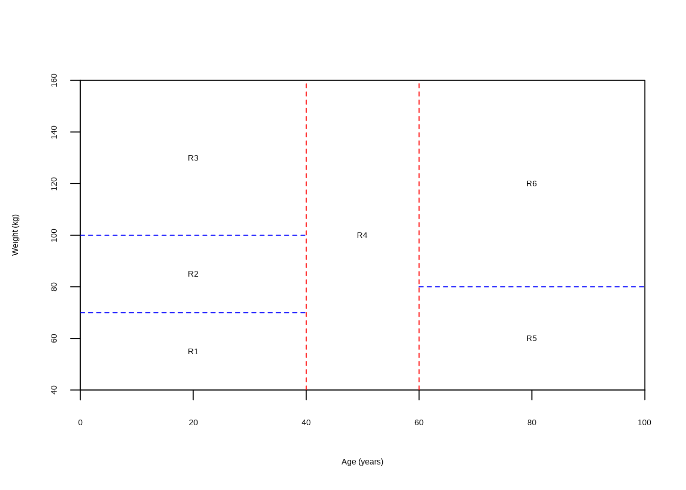
Draw an example (of your own invention) of a partition of two-dimensional feature space that could result from recursive binary splitting. Your example should contain at least six regions. Draw a decision tree corresponding to this partition. Be sure to label all aspects of your figures, including the regions \(R_1, R_2, ...,\) the cutpoints \(t_1, t_2, ...,\) and so forth.
Hint: Your result should look something like Figures 8.1 and 8.2.
tree <- ape::read.tree(text = "(((R1:1,R2:1)N1:2,R3:4)N2:2,(R4:2,(R5:1,R6:1)R3:2)N4:5)R;")
tree$node.label <- c("Age < 40", "Weight < 100", "Weight < 70", "Age < 60", "Weight < 80")

ggtree(tree, ladderize = FALSE) + scale_x_reverse() + coord_flip() +
  geom_tiplab(vjust = 2, hjust = 0.5) +
  geom_text2(aes(label = label, subset = !isTip), hjust = -0.1, vjust = -1)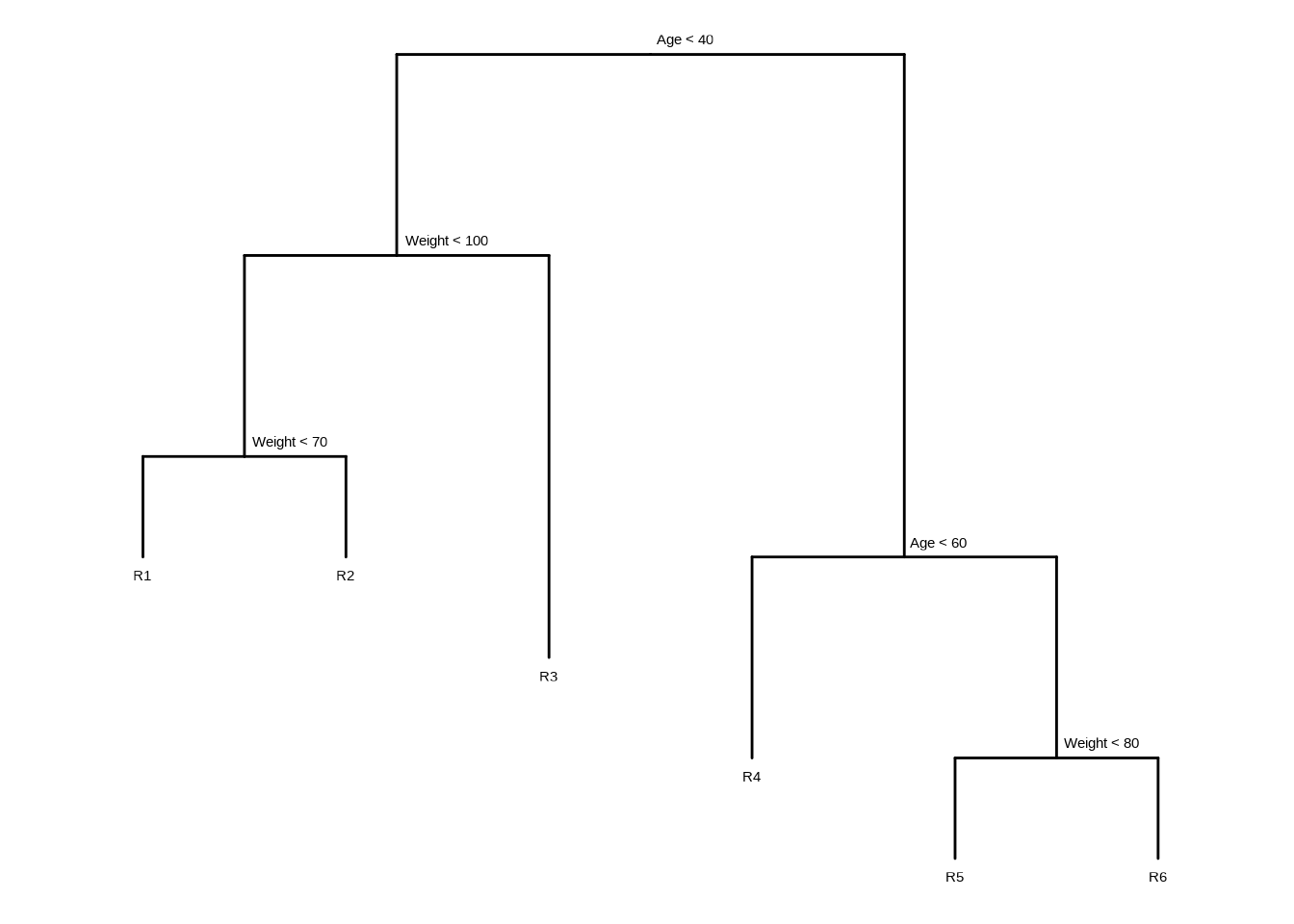
plot(NULL,
  xlab = "Age (years)", ylab = "Weight (kg)",
  xlim = c(0, 100), ylim = c(40, 160), xaxs = "i", yaxs = "i"
)
abline(v = 40, col = "red", lty = 2)
lines(c(0, 40), c(100, 100), col = "blue", lty = 2)
lines(c(0, 40), c(70, 70), col = "blue", lty = 2)
abline(v = 60, col = "red", lty = 2)
lines(c(60, 100), c(80, 80), col = "blue", lty = 2)

text(
  c(20, 20, 20, 50, 80, 80),
  c(55, 85, 130, 100, 60, 120),
  labels = c("R1", "R2", "R3", "R4", "R5", "R6")
)
8.1.2 Question 2
It is mentioned in Section 8.2.3 that boosting using depth-one trees (or stumps) leads to an additive model: that is, a model of the form \[ f(X) = \sum_{j=1}^p f_j(X_j). \] Explain why this is the case. You can begin with (8.12) in Algorithm 8.2.
Equation 8.1 is:
\[ f(x) = \sum_{b=1}^B(\lambda \hat{f}^b(x) \]
where \(\hat{f}^b(x)\) represents the \(b\)th tree with (in this case) 1 split. Since 1-depth trees involve only one variable, and the total function for \(x\) involves adding the outcome for each, this model is an additive. Depth 2 trees would allow for interactions between two variables.
8.1.3 Question 3
Consider the Gini index, classification error, and cross-entropy in a simple classification setting with two classes. Create a single plot that displays each of these quantities as a function of \(\hat{p}_{m1}\). The \(x\)-axis should display \(\hat{p}_{m1}\), ranging from 0 to 1, and the \(y\)-axis should display the value of the Gini index, classification error, and entropy.
Hint: In a setting with two classes, \(\hat{p}_{m1} = 1 - \hat{p}_{m2}\). You could make this plot by hand, but it will be much easier to make in
R.
The Gini index is defined by
\[G = \sum_{k=1}^{K} \hat{p}_{mk}(1 - \hat{p}_{mk})\]
Entropy is given by
\[D = -\sum_{k=1}^{K} \hat{p}_{mk}\log(\hat{p}_{mk})\]
The classification error is
\[E = 1 - \max_k(\hat{p}_{mk})\]
# Function definitions are for when there's two classes only
p <- seq(0, 1, length.out = 100)
data.frame(
  x = p,
  "Gini index" = p * (1 - p) * 2,
  "Entropy" = -(p * log(p) + (1 - p) * log(1 - p)),
  "Classification error" = 1 - pmax(p, 1 - p),
  check.names = FALSE
) |>
  pivot_longer(!x) |>
  ggplot(aes(x = x, y = value, color = name)) +
  geom_line(na.rm = TRUE)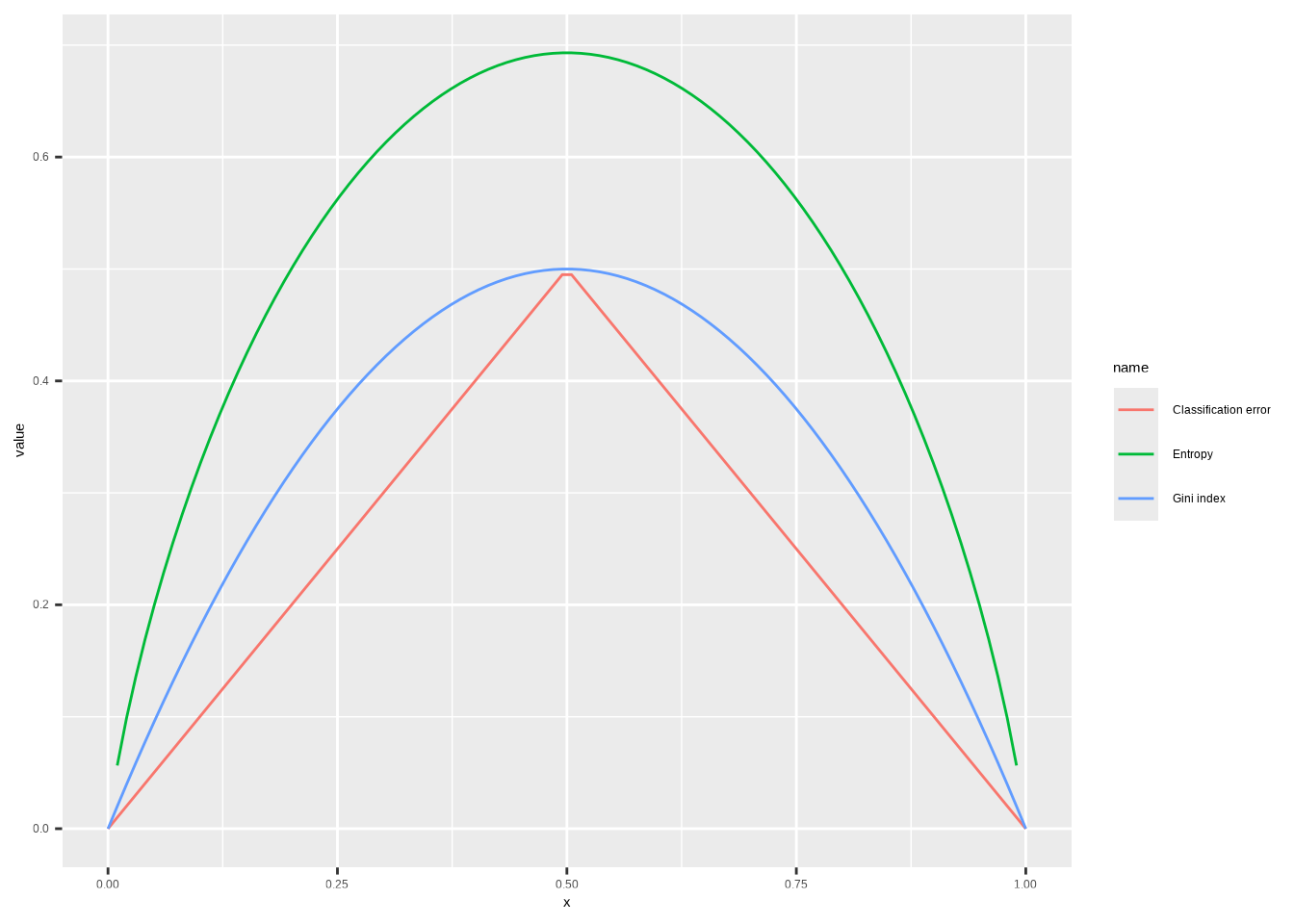
8.1.4 Question 4
This question relates to the plots in Figure 8.12.
- Sketch the tree corresponding to the partition of the predictor space illustrated in the left-hand panel of Figure 8.12. The numbers inside the boxes indicate the mean of \(Y\) within each region.
tree <- ape::read.tree(text = "(((3:1.5,(10:1,0:1)A:1)B:1,15:2)C:1,5:2)D;")
tree$node.label <- c("X1 < 1", "X2 < 1", "X1 < 0", "X2 < 0")

ggtree(tree, ladderize = FALSE) + scale_x_reverse() + coord_flip() +
  geom_tiplab(vjust = 2, hjust = 0.5) +
  geom_text2(aes(label = label, subset = !isTip), hjust = -0.1, vjust = -1)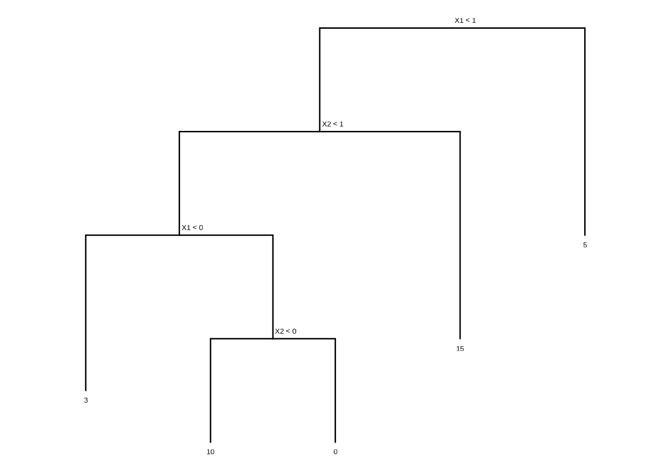
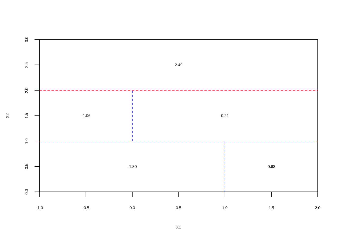
- Create a diagram similar to the left-hand panel of Figure 8.12, using the tree illustrated in the right-hand panel of the same figure. You should divide up the predictor space into the correct regions, and indicate the mean for each region.
plot(NULL, xlab = "X1", ylab = "X2", xlim = c(-1, 2), ylim = c(0, 3), xaxs = "i", yaxs = "i")
abline(h = 1, col = "red", lty = 2)
lines(c(1, 1), c(0, 1), col = "blue", lty = 2)
lines(c(-1, 2), c(2, 2), col = "red", lty = 2)
lines(c(0, 0), c(1, 2), col = "blue", lty = 2)
text(
  c(0, 1.5, -0.5, 1, 0.5),
  c(0.5, 0.5, 1.5, 1.5, 2.5),
  labels = c("-1.80", "0.63", "-1.06", "0.21", "2.49")
)
8.1.5 Question 5
Suppose we produce ten bootstrapped samples from a data set containing red and green classes. We then apply a classification tree to each bootstrapped sample and, for a specific value of \(X\), produce 10 estimates of \(P(\textrm{Class is Red}|X)\): \[0.1, 0.15, 0.2, 0.2, 0.55, 0.6, 0.6, 0.65, 0.7, \textrm{and } 0.75.\] There are two common ways to combine these results together into a single class prediction. One is the majority vote approach discussed in this chapter. The second approach is to classify based on the average probability. In this example, what is the final classification under each of these two approaches?
x <- c(0.1, 0.15, 0.2, 0.2, 0.55, 0.6, 0.6, 0.65, 0.7, 0.75)
ifelse(mean(x > 0.5), "red", "green") # majority vote
## [1] "red"## [1] "green"8.1.6 Question 6
Provide a detailed explanation of the algorithm that is used to fit a regression tree.
First we perform binary recursive splitting of the data, to minimize RSS at each split. This is continued until there are n samples present in each leaf. Then we prune the tree to a set of subtrees determined by a parameter \(\alpha\). Using K-fold CV, we select \(\alpha\) to minimize the cross validation error. The final tree is then calculated using the complete dataset with the selected \(\alpha\) value.
8.2 Applied
8.2.1 Question 7
In the lab, we applied random forests to the
Bostondata usingmtry = 6and usingntree = 25andntree = 500. Create a plot displaying the test error resulting from random forests on this data set for a more comprehensive range of values formtryandntree. You can model your plot after Figure 8.10. Describe the results obtained.
## randomForest 4.7-1.2## Type rfNews() to see new features/changes/bug fixes.##
## Attaching package: 'randomForest'## The following object is masked from 'package:ggtree':
##
## margin## The following object is masked from 'package:dplyr':
##
## combine## The following object is masked from 'package:ggplot2':
##
## marginset.seed(42)
train <- sample(c(TRUE, FALSE), nrow(Boston), replace = TRUE)
rf_err <- function(mtry) {
randomForest(
Boston[train, -13],
y = Boston[train, 13],
xtest = Boston[!train, -13],
ytest = Boston[!train, 13],
mtry = mtry,
ntree = 500
)$test$mse
}
res <- lapply(c(1, 2, 3, 5, 7, 10, 12), rf_err)
names(res) <- c(1, 2, 3, 5, 7, 10, 12)
data.frame(res, check.names = FALSE) |>
mutate(n = 1:500) |>
pivot_longer(!n) |>
ggplot(aes(x = n, y = value, color = name)) +
geom_line(na.rm = TRUE) +
xlab("Number of trees") +
ylab("Error") +
scale_y_log10() +
scale_color_discrete(name = "No. variables at\neach split")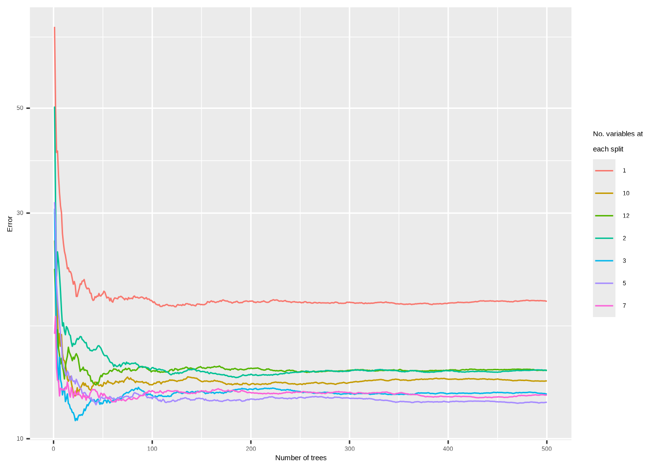
8.2.2 Question 8
In the lab, a classification tree was applied to the
Carseatsdata set after convertingSalesinto a qualitative response variable. Now we will seek to predictSalesusing regression trees and related approaches, treating the response as a quantitative variable.
- Split the data set into a training set and a test set.
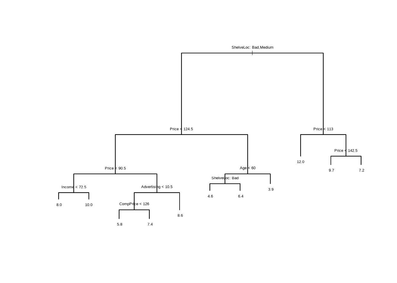
- Fit a regression tree to the training set. Plot the tree, and interpret the results. What test error rate do you obtain?
##
## Regression tree:
## tree(formula = Sales ~ ., data = Carseats[train, ])
## Variables actually used in tree construction:
## [1] "ShelveLoc"   "Price"       "Income"      "Advertising" "CompPrice"
## [6] "Age"
## Number of terminal nodes:  16
## Residual mean deviance:  2.356 = 424.1 / 180
## Distribution of residuals:
##     Min.  1st Qu.   Median     Mean  3rd Qu.     Max.
## -4.54900 -0.82980  0.03075  0.00000  0.89250  4.83100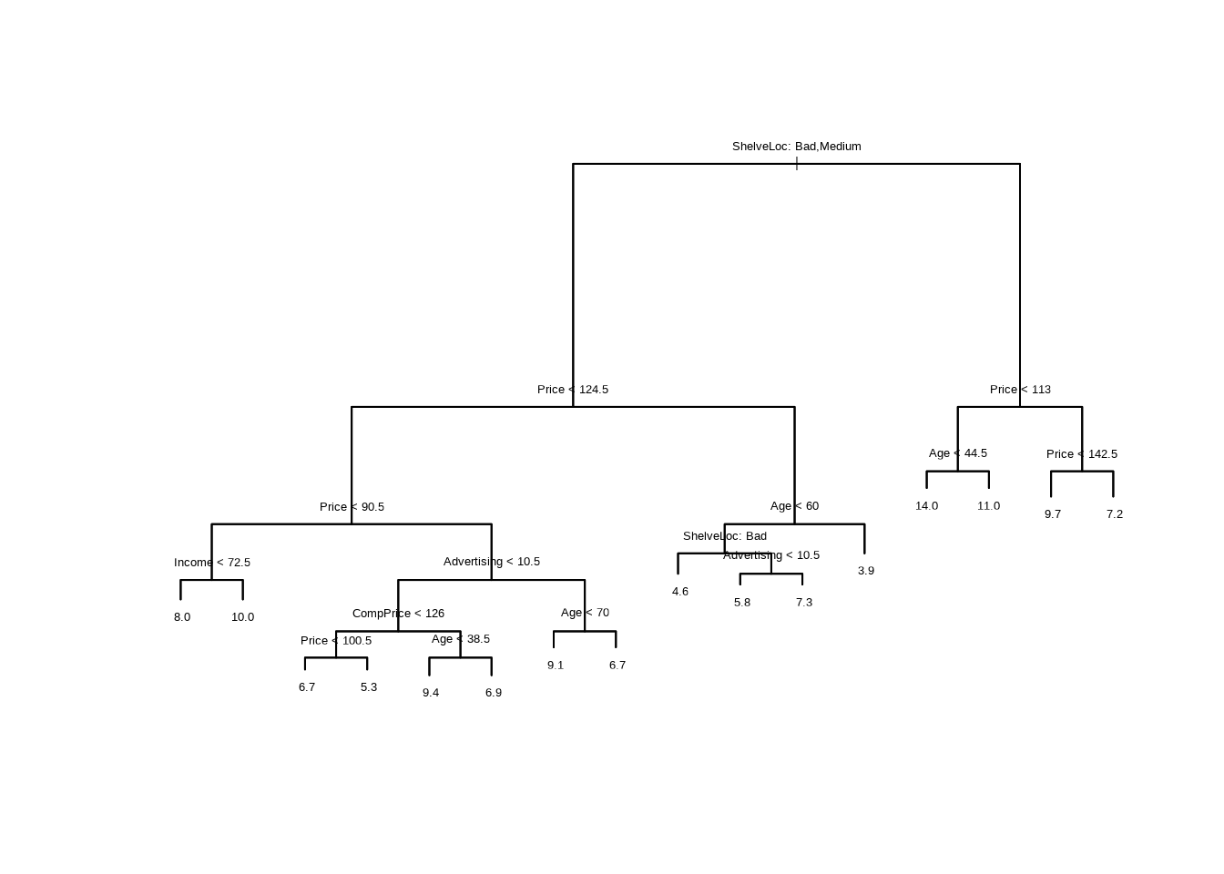
carseats_mse <- function(model) {
  p <- predict(model, newdata = Carseats[!train, ])
  mean((p - Carseats[!train, "Sales"])^2)
}
carseats_mse(tr)
## [1] 4.559764
- Use cross-validation in order to determine the optimal level of tree complexity. Does pruning the tree improve the test error rate?
res <- cv.tree(tr)
plot(res$size, res$dev, type = "b", xlab = "Tree size", ylab = "Deviance")
min <- which.min(res$dev)
abline(v = res$size[min], lty = 2, col = "red")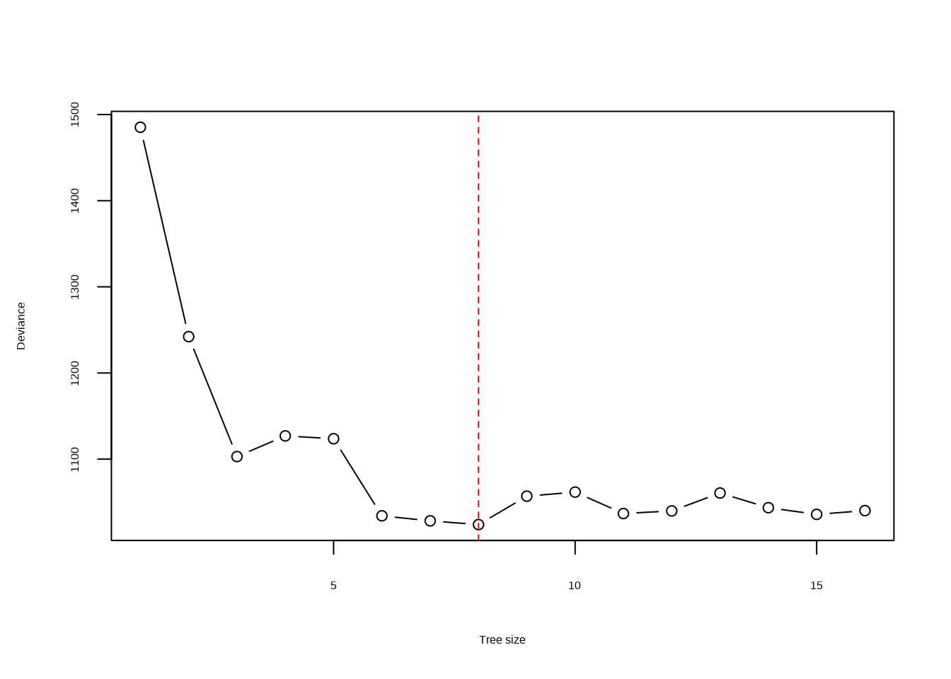
Pruning improves performance very slightly (though this is not repeatable in different rounds of cross-validation). Arguably, a good balance is achieved when the tree size is 11.
## [1] 4.625875
- Use the bagging approach in order to analyze this data. What test error rate do you obtain? Use the
importance()function to determine which variables are most important.
# Here we can use random Forest with mtry = 10 = p (the number of predictor
# variables) to perform bagging
bagged <- randomForest(Sales ~ .,
  data = Carseats[train, ], mtry = 10,
  ntree = 200, importance = TRUE
)
carseats_mse(bagged)
## [1] 2.762861## %IncMSE IncNodePurity
## CompPrice 11.2608998 104.474222
## Income 5.0953983 73.275066
## Advertising 12.9011190 125.886762
## Population 3.4071044 60.095200
## Price 34.6904380 450.952728
## ShelveLoc 33.7059874 374.808575
## Age 7.9101141 143.652934
## Education -2.1154997 32.712444
## Urban 0.9604097 7.029648
## US 3.1336559 6.287048The test error rate is ~2.8 which is a substantial improvement over the pruned regression tree above.
- Use random forests to analyze this data. What test error rate do you obtain? Use the
importance()function to determine which variables are most important. Describe the effect of \(m\), the number of variables considered at each split, on the error rate obtained.
rf <- randomForest(Sales ~ .,
  data = Carseats[train, ], mtry = 3,
  ntree = 500, importance = TRUE
)
carseats_mse(rf)
## [1] 3.439357## %IncMSE IncNodePurity
## CompPrice 8.5717587 122.75189
## Income 2.8955756 116.33951
## Advertising 13.0681194 128.13563
## Population 2.0475415 104.03803
## Price 34.7934136 342.84663
## ShelveLoc 39.0704834 292.56638
## Age 7.7941744 135.69061
## Education 0.8770806 64.67614
## Urban -0.3301478 13.83594
## US 6.2716539 22.07306The test error rate is ~3.0 which is a substantial improvement over the pruned regression tree above, although not quite as good as the bagging approach.
- Now analyze the data using BART, and report your results.
## Loading required package: nlme##
## Attaching package: 'nlme'## The following object is masked from 'package:ggtree':
##
## collapse## The following object is masked from 'package:dplyr':
##
## collapse## Loading required package: survival# For ease, we'll create a fake "predict" method that just returns
# yhat.test.mean regardless of provided "newdata"
predict.wbart <- function(model, ...) model$yhat.test.mean
bartfit <- gbart(Carseats[train, 2:11], Carseats[train, 1],
x.test = Carseats[!train, 2:11]
)## *****Calling gbart: type=1
## *****Data:
## data:n,p,np: 196, 14, 204
## y1,yn: 2.070867, 2.280867
## x1,x[n*p]: 138.000000, 1.000000
## xp1,xp[np*p]: 141.000000, 1.000000
## *****Number of Trees: 200
## *****Number of Cut Points: 58 ... 1
## *****burn,nd,thin: 100,1000,1
## *****Prior:beta,alpha,tau,nu,lambda,offset: 2,0.95,0.287616,3,0.21118,7.42913
## *****sigma: 1.041218
## *****w (weights): 1.000000 ... 1.000000
## *****Dirichlet:sparse,theta,omega,a,b,rho,augment: 0,0,1,0.5,1,14,0
## *****printevery: 100
##
## MCMC
## done 0 (out of 1100)
## done 100 (out of 1100)
## done 200 (out of 1100)
## done 300 (out of 1100)
## done 400 (out of 1100)
## done 500 (out of 1100)
## done 600 (out of 1100)
## done 700 (out of 1100)
## done 800 (out of 1100)
## done 900 (out of 1100)
## done 1000 (out of 1100)
## time: 2s
## trcnt,tecnt: 1000,1000## [1] 1.631285The test error rate is ~1.6 which is an improvement over random forest and bagging.
8.2.3 Question 9
This problem involves the
OJdata set which is part of theISLR2package.
- Create a training set containing a random sample of 800 observations, and a test set containing the remaining observations.
- Fit a tree to the training data, with
Purchaseas the response and the other variables except forBuyas predictors. Use thesummary()function to produce summary statistics about the tree, and describe the results obtained. What is the training error rate? How many terminal nodes does the tree have?
##
## Classification tree:
## tree(formula = Purchase ~ ., data = OJ[train, ])
## Variables actually used in tree construction:
## [1] "LoyalCH"     "SalePriceMM" "PriceDiff"
## Number of terminal nodes:  8
## Residual mean deviance:  0.7392 = 585.5 / 792
## Misclassification error rate: 0.1638 = 131 / 800
- Type in the name of the tree object in order to get a detailed text output. Pick one of the terminal nodes, and interpret the information displayed.
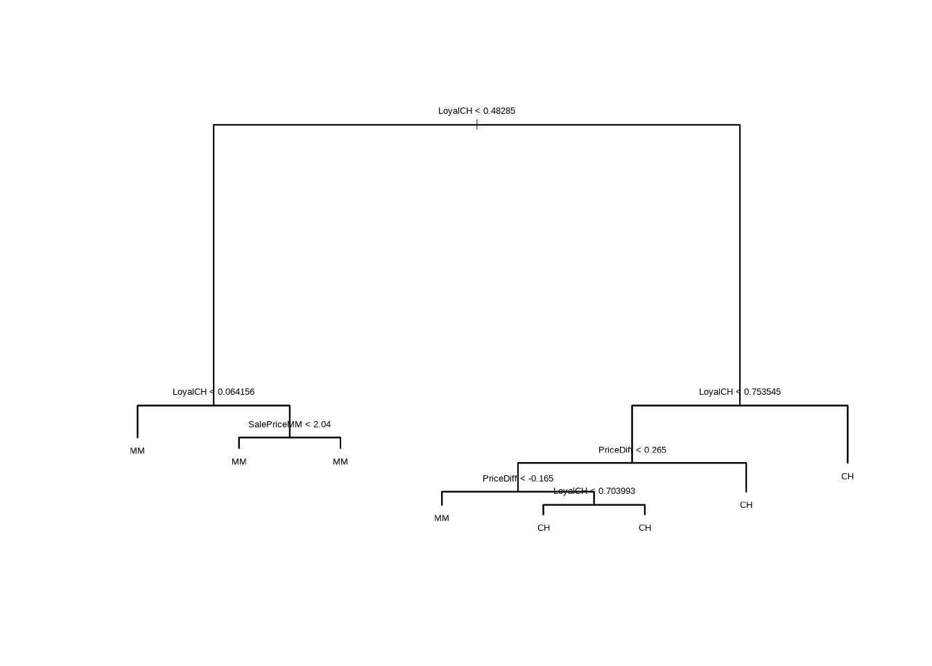
## node), split, n, deviance, yval, (yprob)
##       * denotes terminal node
##
##  1) root 800 1066.00 CH ( 0.61500 0.38500 )
##    2) LoyalCH < 0.48285 285  296.00 MM ( 0.21404 0.78596 )
##      4) LoyalCH < 0.064156 64    0.00 MM ( 0.00000 1.00000 ) *
##      5) LoyalCH > 0.064156 221  260.40 MM ( 0.27602 0.72398 )
##       10) SalePriceMM < 2.04 128  123.50 MM ( 0.18750 0.81250 ) *
##       11) SalePriceMM > 2.04 93  125.00 MM ( 0.39785 0.60215 ) *
##    3) LoyalCH > 0.48285 515  458.10 CH ( 0.83689 0.16311 )
##      6) LoyalCH < 0.753545 230  282.70 CH ( 0.69565 0.30435 )
##       12) PriceDiff < 0.265 149  203.00 CH ( 0.57718 0.42282 )
##         24) PriceDiff < -0.165 32   38.02 MM ( 0.28125 0.71875 ) *
##         25) PriceDiff > -0.165 117  150.30 CH ( 0.65812 0.34188 )
##           50) LoyalCH < 0.703993 105  139.60 CH ( 0.61905 0.38095 ) *
##           51) LoyalCH > 0.703993 12    0.00 CH ( 1.00000 0.00000 ) *
##       13) PriceDiff > 0.265 81   47.66 CH ( 0.91358 0.08642 ) *
##      7) LoyalCH > 0.753545 285  111.70 CH ( 0.95088 0.04912 ) *
- Create a plot of the tree, and interpret the results.
- Predict the response on the test data, and produce a confusion matrix comparing the test labels to the predicted test labels. What is the test error rate?
##
##       CH  MM
##   CH 125  15
##   MM  36  94
- Apply the
cv.tree()function to the training set in order to determine the optimal tree size.
- Produce a plot with tree size on the \(x\)-axis and cross-validated classification error rate on the \(y\)-axis.
plot(res$size, res$dev, type = "b", xlab = "Tree size", ylab = "Deviance")
min <- which.min(res$dev)
abline(v = res$size[min], lty = 2, col = "red")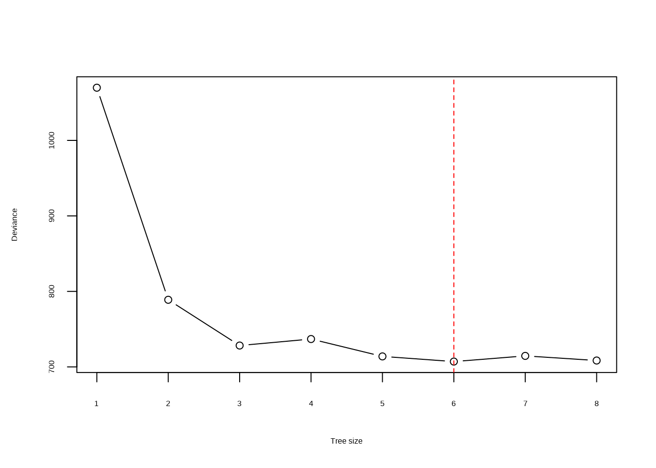
- Which tree size corresponds to the lowest cross-validated classification error rate?
## [1] 6
- Produce a pruned tree corresponding to the optimal tree size obtained using cross-validation. If cross-validation does not lead to selection of a pruned tree, then create a pruned tree with five terminal nodes.
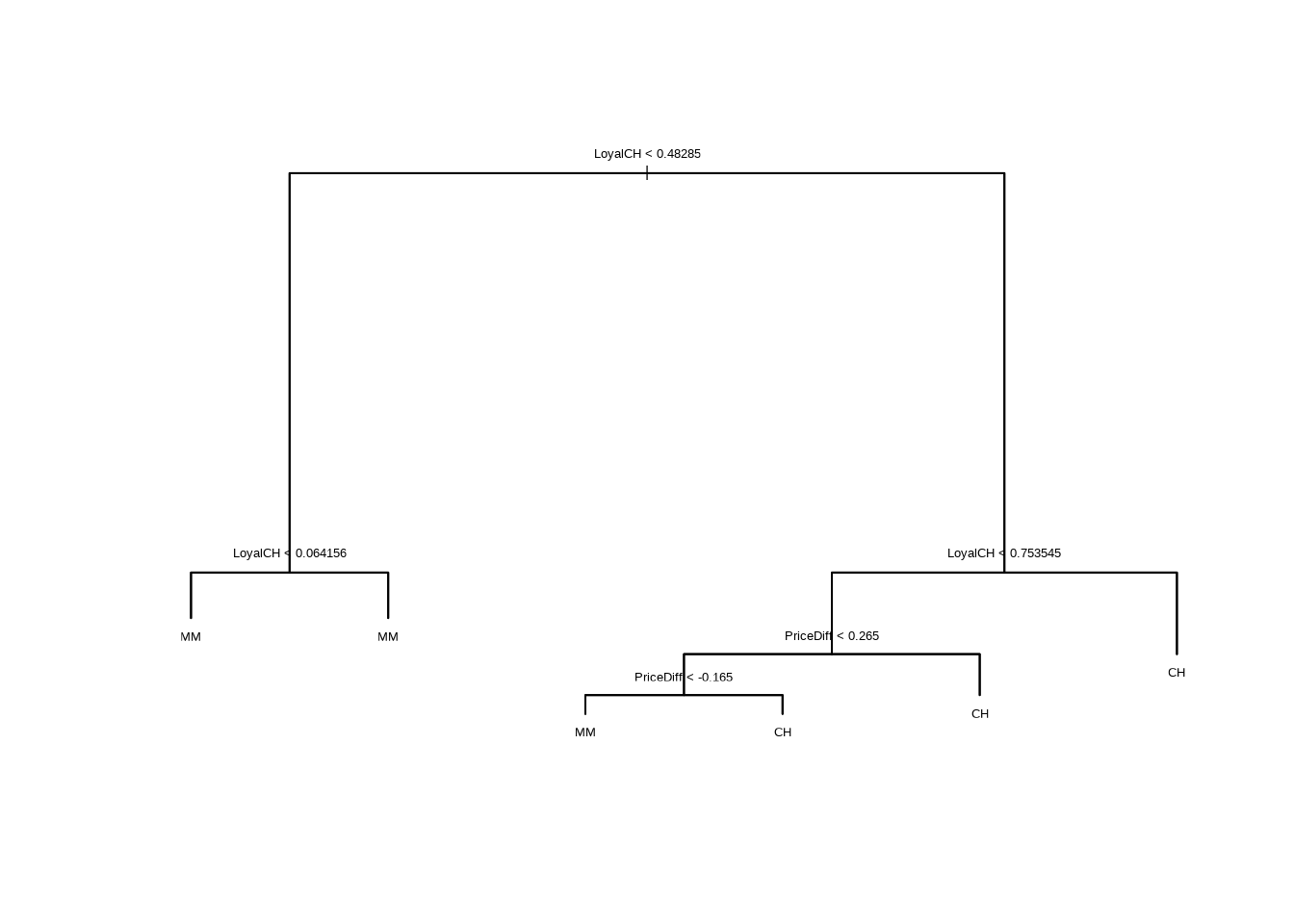
- Compare the training error rates between the pruned and unpruned trees. Which is higher?
oj_misclass <- function(model) {
  summary(model)$misclass[1] / summary(model)$misclass[2]
}
oj_misclass(tr)
## [1] 0.16375## [1] 0.16375The training misclassification error rate is slightly higher for the pruned tree.
- Compare the test error rates between the pruned and unpruned trees. Which is higher?
oj_err <- function(model) {
  p <- predict(model, newdata = OJ[test, ], type = "class")
  mean(p != OJ[test, "Purchase"])
}
oj_err(tr)
## [1] 0.1888889## [1] 0.1888889The test misclassification error rate is slightly higher for the pruned tree.
8.2.4 Question 10
We now use boosting to predict
Salaryin theHittersdata set.
- Remove the observations for whom the salary information is unknown, and then log-transform the salaries.
- Create a training set consisting of the first 200 observations, and a test set consisting of the remaining observations.
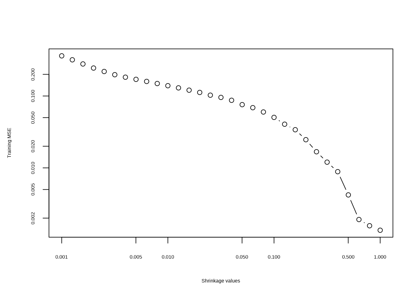
- Perform boosting on the training set with 1,000 trees for a range of values of the shrinkage parameter \(\lambda\). Produce a plot with different shrinkage values on the \(x\)-axis and the corresponding training set MSE on the \(y\)-axis.
## Loaded gbm 2.2.2## This version of gbm is no longer under development. Consider transitioning to gbm3, https://github.com/gbm-developers/gbm3set.seed(42)
lambdas <- 10^seq(-3, 0, by = 0.1)
fits <- lapply(lambdas, function(lam) {
gbm(Salary ~ .,
data = dat[train, ], distribution = "gaussian",
n.trees = 1000, shrinkage = lam
)
})
errs <- sapply(fits, function(fit) {
p <- predict(fit, dat[train, ], n.trees = 1000)
mean((p - dat[train, ]$Salary)^2)
})
plot(lambdas, errs,
type = "b", xlab = "Shrinkage values",
ylab = "Training MSE", log = "xy"
)
- Produce a plot with different shrinkage values on the \(x\)-axis and the corresponding test set MSE on the \(y\)-axis.
errs <- sapply(fits, function(fit) {
  p <- predict(fit, dat[test, ], n.trees = 1000)
  mean((p - dat[test, ]$Salary)^2)
})
plot(lambdas, errs,
  type = "b", xlab = "Shrinkage values",
  ylab = "Training MSE", log = "xy"
)
min(errs)
## [1] 0.249881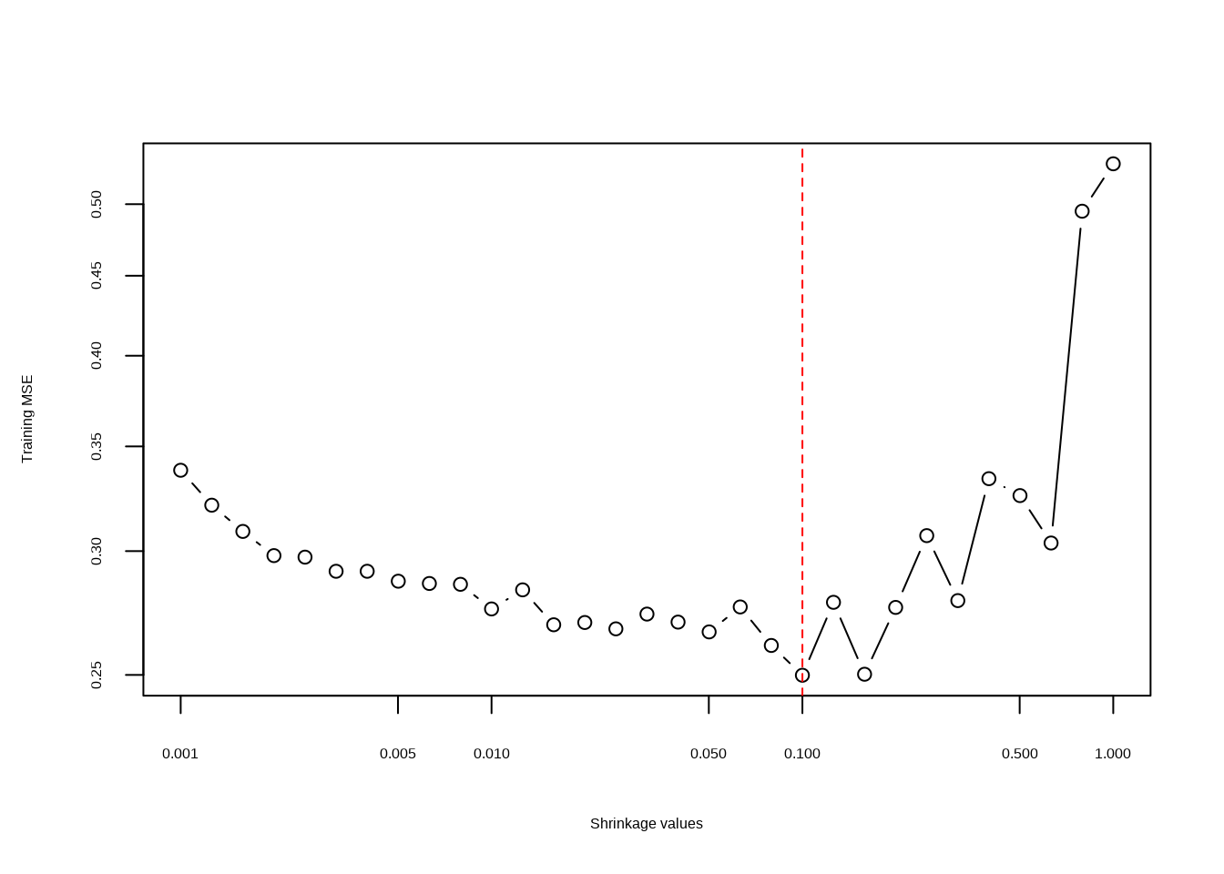
- Compare the test MSE of boosting to the test MSE that results from applying two of the regression approaches seen in Chapters 3 and 6.
Linear regression
fit1 <- lm(Salary ~ ., data = dat[train, ])
mean((predict(fit1, dat[test, ]) - dat[test, "Salary"])^2)
## [1] 0.4917959Ridge regression
## Loading required package: Matrix##
## Attaching package: 'Matrix'## The following object is masked from 'package:ggtree':
##
## expand## The following objects are masked from 'package:tidyr':
##
## expand, pack, unpack## Loaded glmnet 4.1-8x <- model.matrix(Salary ~ ., data = dat[train, ])
x.test <- model.matrix(Salary ~ ., data = dat[test, ])
y <- dat[train, "Salary"]
fit2 <- glmnet(x, y, alpha = 1)
mean((predict(fit2, s = 0.1, newx = x.test) - dat[test, "Salary"])^2)## [1] 0.4389054
- Which variables appear to be the most important predictors in the boosted model?
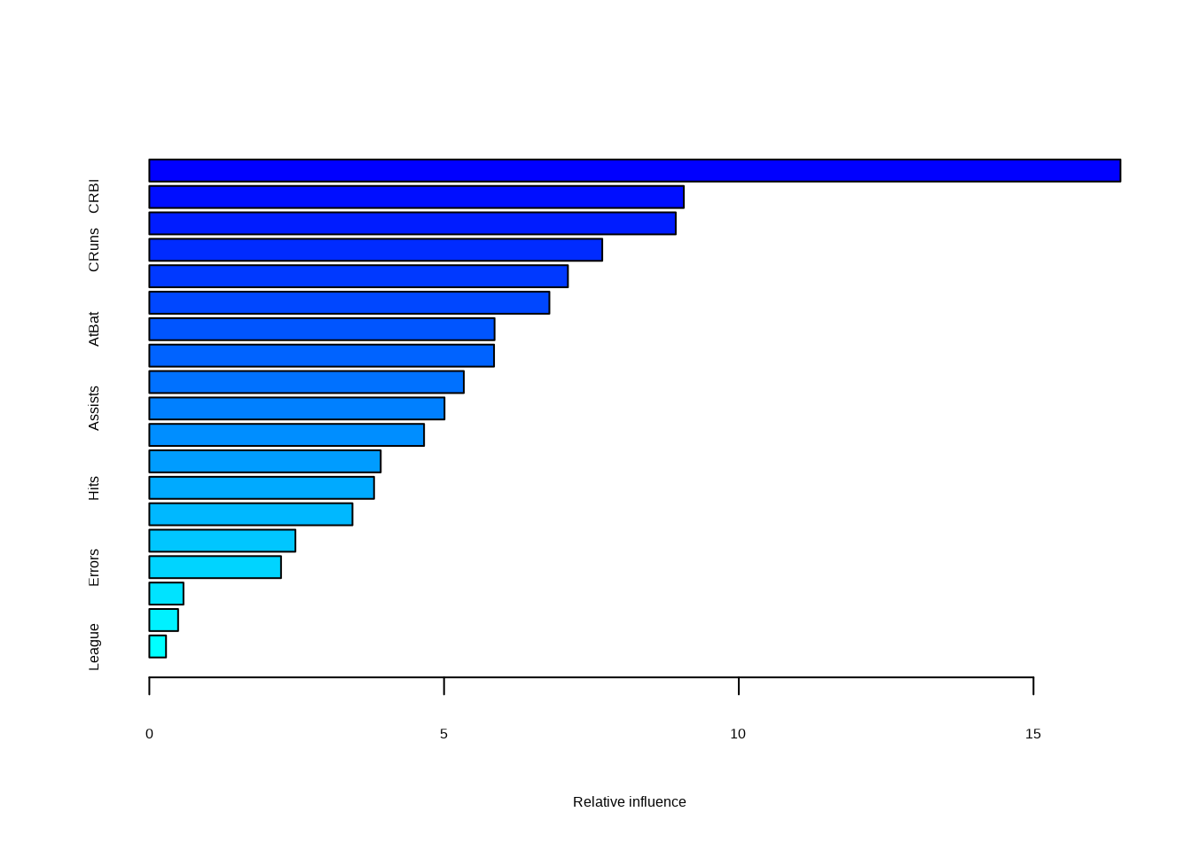
##                 var    rel.inf
## CAtBat       CAtBat 16.4755242
## CRBI           CRBI  9.0670759
## CHits         CHits  8.9307168
## CRuns         CRuns  7.6839786
## CWalks       CWalks  7.1014886
## PutOuts     PutOuts  6.7869382
## AtBat         AtBat  5.8567916
## Walks         Walks  5.8479836
## Years         Years  5.3349489
## Assists     Assists  5.0076392
## CHmRun       CHmRun  4.6606919
## RBI             RBI  3.9255396
## Hits           Hits  3.8123124
## HmRun         HmRun  3.4462640
## Runs           Runs  2.4779866
## Errors       Errors  2.2341326
## NewLeague NewLeague  0.5788283
## Division   Division  0.4880237
## League       League  0.2831352
- Now apply bagging to the training set. What is the test set MSE for this approach?
set.seed(42)
bagged <- randomForest(Salary ~ ., data = dat[train, ], mtry = 19, ntree = 1000)
mean((predict(bagged, newdata = dat[test, ]) - dat[test, "Salary"])^2)
## [1] 0.22788138.2.5 Question 11
This question uses the
Caravandata set.
- Create a training set consisting of the first 1,000 observations, and a test set consisting of the remaining observations.
- Fit a boosting model to the training set with
Purchaseas the response and the other variables as predictors. Use 1,000 trees, and a shrinkage value of 0.01. Which predictors appear to be the most important?
set.seed(42)
fit <- gbm(as.numeric(Purchase == "Yes") ~ ., data = Caravan[train, ], n.trees = 1000, shrinkage = 0.01)
## Distribution not specified, assuming bernoulli ...## Warning in gbm.fit(x = x, y = y, offset = offset, distribution = distribution,
## : variable 50: PVRAAUT has no variation.## Warning in gbm.fit(x = x, y = y, offset = offset, distribution = distribution,
## : variable 71: AVRAAUT has no variation.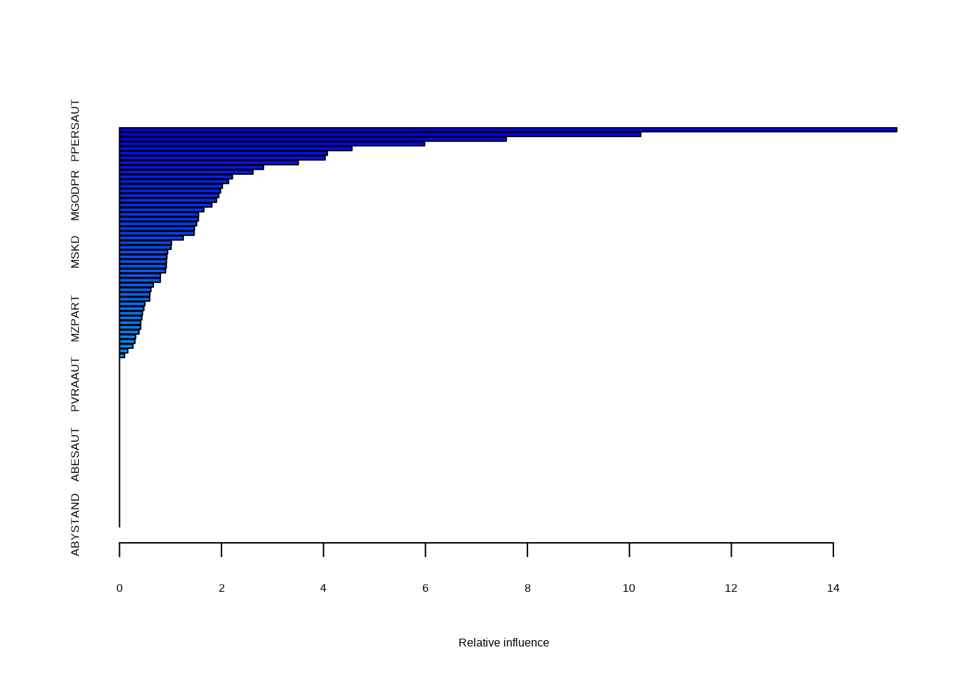
##               var   rel.inf
## PPERSAUT PPERSAUT 15.243041
## MKOOPKLA MKOOPKLA 10.220498
## MOPLHOOG MOPLHOOG  7.584734
## MBERMIDD MBERMIDD  5.983650
## PBRAND     PBRAND  4.557491
## ABRAND     ABRAND  4.076017
- Use the boosting model to predict the response on the test data. Predict that a person will make a purchase if the estimated probability of purchase is greater than 20%. Form a confusion matrix. What fraction of the people predicted to make a purchase do in fact make one? How does this compare with the results obtained from applying KNN or logistic regression to this data set?
p <- predict(fit, Caravan[test, ], n.trees = 1000, type = "response")
table(p > 0.2, Caravan[test, "Purchase"] == "Yes")
##
## FALSE TRUE
## FALSE 4415 257
## TRUE 118 32## [1] 0.2133333141 (109 + 32) are predicted to purchase. Of these 32 do which is 21%.
# Logistic regression
fit <- glm(Purchase == "Yes" ~ ., data = Caravan[train, ], family = "binomial")
## Warning: glm.fit: fitted probabilities numerically 0 or 1 occurred## Warning in predict.lm(object, newdata, se.fit, scale = 1, type = if (type == :
## prediction from rank-deficient fit; attr(*, "non-estim") has doubtful cases##
## FALSE TRUE
## FALSE 4183 231
## TRUE 350 58## [1] 0.1421569For logistic regression we correctly predict 14% of those predicted to purchase.
library(class)
# KNN
fit <- knn(Caravan[train, -86], Caravan[test, -86], Caravan$Purchase[train])
table(fit, Caravan[test, "Purchase"] == "Yes")
##
## fit FALSE TRUE
## No 4260 263
## Yes 273 26## [1] 0.08695652For KNN we correctly predict 8.7% of those predicted to purchase.
8.2.6 Question 12
Apply boosting, bagging, random forests and BART to a data set of your choice. Be sure to fit the models on a training set and to evaluate their performance on a test set. How accurate are the results compared to simple methods like linear or logistic regression? Which of these approaches yields the best performance?
Here I’m going to use the College dataset (used in Question 10 from Chapter 7
to compare performance with the GAM we previously built). In this model we
were trying to predict Outstate using the other variables in College.
## Loading required package: splines## Loading required package: foreach##
## Attaching package: 'foreach'## The following objects are masked from 'package:purrr':
##
## accumulate, when## Loaded gam 1.22-5set.seed(42)
train <- sample(1:nrow(College), 400)
test <- setdiff(1:nrow(College), train)
# Linear regression
lr <- gam(Outstate ~ ., data = College[train, ])
# GAM from chapter 7
gam <- gam(Outstate ~ Private + s(Room.Board, 2) + s(PhD, 2) +
s(perc.alumni, 2) + s(Expend, 2) + s(Grad.Rate, 2), data = College[train, ])
# Boosting
boosted <- gbm(Outstate ~ ., data = College[train, ], n.trees = 1000, shrinkage = 0.01)## Distribution not specified, assuming gaussian ...# Bagging (random forest with mtry = no. predictors)
bagged <- randomForest(Outstate ~ ., data = College[train, ], mtry = 17, ntree = 1000)
# Random forest with mtry = sqrt(no. predictors)
rf <- randomForest(Outstate ~ ., data = College[train, ], mtry = 4, ntree = 1000)
# BART
pred <- setdiff(colnames(College), "Outstate")
bart <- gbart(College[train, pred], College[train, "Outstate"],
x.test = College[test, pred]
)## *****Calling gbart: type=1
## *****Data:
## data:n,p,np: 400, 18, 377
## y1,yn: -4030.802500, 77.197500
## x1,x[n*p]: 1.000000, 71.000000
## xp1,xp[np*p]: 0.000000, 99.000000
## *****Number of Trees: 200
## *****Number of Cut Points: 1 ... 75
## *****burn,nd,thin: 100,1000,1
## *****Prior:beta,alpha,tau,nu,lambda,offset: 2,0.95,301.581,3,715815,10580.8
## *****sigma: 1916.969943
## *****w (weights): 1.000000 ... 1.000000
## *****Dirichlet:sparse,theta,omega,a,b,rho,augment: 0,0,1,0.5,1,18,0
## *****printevery: 100
##
## MCMC
## done 0 (out of 1100)
## done 100 (out of 1100)
## done 200 (out of 1100)
## done 300 (out of 1100)
## done 400 (out of 1100)
## done 500 (out of 1100)
## done 600 (out of 1100)
## done 700 (out of 1100)
## done 800 (out of 1100)
## done 900 (out of 1100)
## done 1000 (out of 1100)
## time: 4s
## trcnt,tecnt: 1000,1000mse <- function(model, ...) {
pred <- predict(model, College[test, ], ...)
mean((College$Outstate[test] - pred)^2)
}
res <- c(
"Linear regression" = mse(lr),
"GAM" = mse(gam),
"Boosting" = mse(boosted, n.trees = 1000),
"Bagging" = mse(bagged),
"Random forest" = mse(rf),
"BART" = mse(bart)
)
res <- data.frame("MSE" = res)
res$Model <- factor(row.names(res), levels = rev(row.names(res)))
ggplot(res, aes(Model, MSE)) +
coord_flip() +
geom_bar(stat = "identity", fill = "steelblue")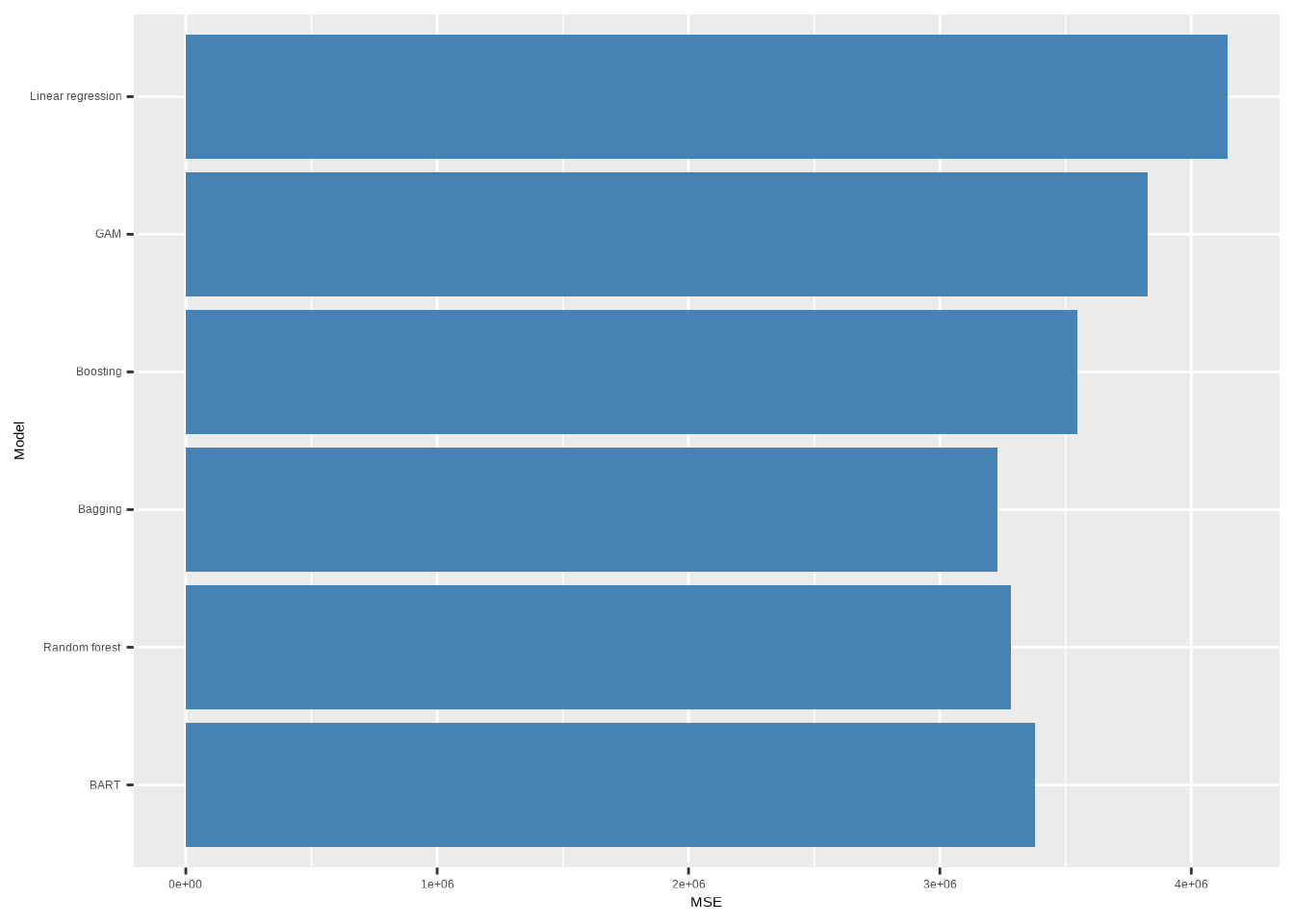
In this case, it looks like bagging produces the best performing model in terms of test mean square error.